
Regression Diagnostics: Residuals, Leverage, Influence, Python, R, SPSS and Excel Guide
Regression Diagnostics evaluates whether a fitted regression equation is trustworthy, where it fails, and which observations have enough residual, leverage, or deletion influence to change the interpretation. This worked guide audits a 649-case OLS model for G3 using six predictors, exact thresholds, ten Python charts, four R charts, SPSS output, and a worked Excel review.
Regression Diagnostics Model Overview
Regression Diagnostics is the structured examination of residual behavior, predictor-space geometry, case-deletion influence, collinearity, functional form, variance, and dependence after a regression model has been fitted. A high R² does not make this review optional. A model can explain much of the observed outcome variation and still have heteroscedastic errors, severe boundary failures, unstable coefficients, or influential cases that dominate selected conclusions.
The worked model predicts the final grade G3 from G1, G2, studytime, failures, absences, and age. All 649 rows are complete for these fields. The fitted equation has R² = 0.850632, adjusted R² = 0.849236, and RMSE = 1.254409. Those values indicate strong fitted-sample performance, but Regression Diagnostics reveals statistically and practically important weaknesses in functional form, residual tails, variance, and individual-case sensitivity.
What Is Regression Diagnostics?
Regression Diagnostics is not one test and is not one graph. The residual-versus-fitted plot evaluates mean form and spread. The Q–Q plot and histogram describe residual shape. Leverage measures predictor-space extremity. Cook’s distance, DFFITS, and COVRATIO measure different consequences of deleting a case. Ramsey RESET, Breusch–Pagan, White, Shapiro–Wilk, Jarque–Bera, Durbin–Watson, VIF, and tolerance add formal or numerical evidence.
The methods are connected but not interchangeable. A case can have very high leverage and a modest residual, as case 1 does. Another case can have a catastrophic residual but ordinary leverage, as case 173 does. Case 164 combines both dimensions and therefore becomes the strongest influence concern. Regression Diagnostics is most informative when each observation is described by its complete profile rather than by one label.
When Should Regression Diagnostics Be Used?
Required uses
- Before interpreting OLS coefficients, confidence intervals, or prediction accuracy.
- When the outcome has boundaries, spikes, floor effects, or ceiling effects.
- When predictor combinations may be unusual or sparse.
- When a model contains correlated predictors, transformations, or interactions.
- When conclusions could change after deleting one observation or a small group.
- When standard errors and p-values are used for decisions.
Common mistakes
- Reporting only R² and assuming the model is adequate.
- Deleting every case beyond a heuristic cutoff.
- Calling high leverage an outcome outlier.
- Treating Cook’s 4/n rule as a formal significance test.
- Using a Q–Q plot without checking variance and influence.
- Changing the model until all diagnostic p-values become nonsignificant.
Regression Diagnostics Model Formula
The fitted value is the model’s predicted conditional mean. The raw residual is eᵢ = yᵢ − ŷᵢ. The diagnostic calculations use the six slopes plus the intercept, so the parameter count is p = 7 even though the number of predictors is k = 6.
Compares a deleted-case residual with a leave-one-out scale and leverage adjustment. The screen is |rᵢ| > 3.
The diagonal hᵢᵢ of the hat matrix. The worked screen is 2p/n = 0.021572.
Combines residual size and leverage to summarize coefficient-vector change. The screen is 4/n = 0.006163.
Measures change in a case’s fitted value after deletion. The screen is 2√(p/n) = 0.207710.
Measures change in generalized coefficient covariance. The worked acceptable band is 0.967643 to 1.032357.
Summarize predictor collinearity. The highest VIF is 4.154857 and the lowest tolerance is 0.240682.
Regression Diagnostics Assumptions and Requirements
1. Correct outcome and conditional-mean form
The OLS equation should be a defensible approximation to E(G3|X). A significant RESET result suggests that omitted nonlinear terms, interactions, or a different model family should be considered.
2. Independent observational units
Residual calculations assume the rows represent independent units unless the model explicitly accounts for clusters or repeated measurements. Durbin–Watson is not a substitute for understanding the sampling design.
3. Finite and meaningful predictor values
Leverage and influence depend on the exact predictor matrix. Recoding, rescaling, adding interactions, or changing the complete-case sample changes the hat matrix and all related thresholds.
4. Constant variance for ordinary OLS inference
Homoscedastic residuals are required for the usual OLS covariance formula. When variance changes, robust standard errors or a better variance model should be evaluated.
5. Approximately normal residuals for small-sample tests
Point estimates do not require normal predictors. Residual normality mainly supports conventional small-sample t and F inference. In a large sample, visual tail severity and influence matter alongside formal tests.
6. Valid observations are not automatically removable
A diagnostic flag means “investigate and compare,” not “delete.” Removal requires a verified error, an ineligible unit, or a prespecified population rule.
Current Worked Scenario
The current Regression Diagnostics casebook uses 649 observations, a continuous G3 outcome, six numeric predictors, and one intercept. Sixty-two observations cross at least one residual, leverage, Cook, DFFITS, or COVRATIO screen. Ten are deleted-residual outliers, 45 exceed the leverage screen, 26 exceed Cook’s 4/n screen, 26 exceed the DFFITS screen, and 49 fall outside the COVRATIO band.
Quick Answer
Global Regression Diagnostics
The fitted model is strong in aggregate but does not satisfy every conventional diagnostic condition.
- R² = 0.850632
- Adjusted R² = 0.849236
- RMSE = 1.254409
- RESET p = 0.001085
- Breusch–Pagan p = 0.000010
- White p = 0.00000175
Casewise Regression Diagnostics
A small set has much greater influence than the average observation.
- Case 164: five flags
- rstudent = −7.590715
- leverage = 0.022859
- Cook’s D = 0.176952
- DFFITS = −1.160994
- COVRATIO = 0.566377
Table of Contents
- Why this analysis needs Regression Diagnostics
- How Regression Diagnostics works
- Variables used, coding and sample definition
- Regression Diagnostics results
- Ten Python chart stories
- R charts and explanations
- Diagnostic parameter interpretation
- Predictions, influence and model meaning
- Assumptions and diagnostic decisions
- Python, R, SPSS and Excel workflows
- Code
- Advanced Regression Diagnostics topics
- APA-style reporting
- Publication checklist
- Downloads and chart resources
- Related Salar Cafe guides
- Frequently asked questions
- Regression Diagnostics conclusion
Why This Analysis Needs Regression Diagnostics
The model predicts G3 well for much of the sample, especially where observed grades are concentrated. Without Regression Diagnostics, that central alignment could encourage an overly broad statement that the equation works equally well for every grade profile. The case table shows otherwise. Several students with observed G3 = 0 receive predictions from about 5.48 to 9.02, creating large negative residuals and much of the non-normal lower tail.
Regression Diagnostics is also needed because unusual predictors and unusual outcomes are not the same phenomenon. Case 1 has the largest leverage, 0.103309, but its externally studentized residual is only 0.944918. Case 173 has ordinary leverage, 0.007263, but an extreme externally studentized residual of −7.545231. Case 164 has both a severe error and above-threshold leverage, producing the largest Cook’s distance and DFFITS.
Questions the analysis answers
- Does the residual cloud suggest curvature or omitted structure?
- Does residual variance change across the fitted range?
- Are tails severe enough to affect conventional inference?
- Which observations occupy unusual predictor-space positions?
- Which deletions change fitted values or the coefficient vector most?
- Do predictor correlations make individual slopes unstable?
Questions it does not answer alone
- Whether a flagged observation is a data error.
- Whether deletion is scientifically justified.
- Which nonlinear form is substantively correct.
- Whether future prediction will match fitted-sample accuracy.
- Whether clustered observations are independent.
- Whether coefficient associations are causal effects.
The best use of Regression Diagnostics is a documented comparison workflow: preserve the original analysis, identify each concern, verify cases against source records, fit defensible alternatives, compare conclusions, and explain any dependence on influential observations. This approach protects against both careless deletion and careless acceptance.
How Regression Diagnostics Works
Define G3, the six predictors, complete cases, intercept, and case numbering once.
Calculate fitted values, residual variants, leverage, Cook’s D, DFFITS, and COVRATIO.
Combine plots, formal tests, case review, robust inference, and sensitivity models.
Residual and Influence Formulas
The raw residual retains the outcome unit. A residual of −9 means the observed G3 is nine grade points below the model prediction.
Leverage is determined only by the predictor design. Its average is p/n = 7/649 ≈ 0.010786. The selected screen doubles that average.
The externally studentized residual uses a scale estimate with case i deleted. It is more suitable than a raw residual for comparing observations with different leverage.
Cook’s distance increases when a case combines a large residual with strategic leverage. The exact software calculation should be used rather than a rounded hand formula.
DFFITS focuses on the change in a fitted value, while Cook’s distance summarizes change in the coefficient vector. COVRATIO asks how coefficient precision volume changes.
Exact Regression Diagnostics Thresholds
| Diagnostic | Formula or rule | Exact worked cutoff | Flag count | Use |
|---|---|---|---|---|
| Externally studentized residual | |rstudent| > 3 | 3.000000 | 10 | Conditional outcome outliers |
| Leverage | hᵢᵢ > 2p/n | 0.02157165 | 45 | Unusual predictor profiles |
| Cook’s distance | Dᵢ > 4/n | 0.00616333 | 26 | Coefficient-vector sensitivity |
| DFFITS | |DFFITS| > 2√(p/n) | 0.20770965 | 26 | Fitted-value sensitivity |
| COVRATIO lower | < 1 − 3p/n | 0.96764253 | 49 outside band | Coefficient-covariance sensitivity |
| COVRATIO upper | > 1 + 3p/n | 1.03235747 |
Variables Used, Coding and Sample Definition
| Variable | Role | Definition | Diagnostic implication |
|---|---|---|---|
| G3 | Outcome | Final course grade, with observed boundary values including 0. | Lower-boundary observations create the strongest negative residuals. |
| G1 | Predictor | First-period grade. | VIF = 4.154857; correlated strongly with G2. |
| G2 | Predictor | Second-period grade. | VIF = 4.091388; correlated strongly with G1. |
| studytime | Predictor | Weekly study-time category treated numerically. | VIF = 1.088056; low collinearity contribution. |
| failures | Predictor | Number of previous class failures. | VIF = 1.306096; extreme profiles can contribute to leverage. |
| absences | Predictor | Absence count. | VIF = 1.048621; large counts can create predictor-space extremity. |
| age | Predictor | Age in years. | VIF = 1.154871; high ages appear in some leverage profiles. |
| case_number | Identifier | Sequential diagnostic row number from 1 through 649. | Must remain consistent across tables, labels, and charts. |
The complete-case filter is applied to G3 and the six predictors before model fitting. No categorical dummy variables are used in this equation. The intercept is included, producing p = 7 model parameters. All diagnostic thresholds and leverage values therefore depend on this exact design matrix.
The VIF table is calculated for the six predictors. G1 and G2 have moderate overlap but remain below a commonly used VIF screen of 5. Their tolerances are about 0.241 and 0.244. The other four VIF values are close to 1. Regression Diagnostics therefore identifies moderate grade-predictor overlap rather than severe generalized multicollinearity.
Regression Diagnostics Results
Complete cases
Plus one intercept
Fitted outcome variance
Fit adjusted for parameters
Residual scale in G3 units
Scaled predictor matrix
Flag Counts and Maximum Values
| Screen | Cases flagged | Percentage of 649 | Maximum observed value |
|---|---|---|---|
| Any of five diagnostic rules | 62 | 9.55% | Five flags on case 164 |
| Externally studentized residual | 10 | 1.54% | |7.590715| |
| Leverage | 45 | 6.93% | 0.103309 |
| Cook’s distance | 26 | 4.01% | 0.176952 |
| DFFITS | 26 | 4.01% | |1.160994| |
| COVRATIO outside band | 49 | 7.55% | 0.561339 to 1.116514 among leading cases |
The category counts overlap. They should not be added. The union is 62 observations because many leading cases cross three, four, or five rules. Regression Diagnostics uses the flag count only to organize review; a five-flag case is not five times as problematic as a one-flag case.
Formal Model Checks
| Diagnostic | Statistic | p value | Question | Worked interpretation |
|---|---|---|---|---|
| Ramsey RESET | 10.774057 | 0.001085 | Does the linear mean omit structure? | Evidence of possible functional-form misspecification. |
| Shapiro–Wilk | 0.754697 | 6.2445×10⁻³⁰ | Are residuals normally shaped? | Strong tail departure; inspect magnitude and influence. |
| Jarque–Bera | 10152.729452 | < 0.001 | Do skewness and kurtosis match normality? | Strong non-normality evidence. |
| Breusch–Pagan | 33.054192 | 1.0237×10⁻⁵ | Is variance constant in a linear variance screen? | Evidence of heteroscedasticity. |
| White test | 75.547435 | 1.7529×10⁻⁶ | Is variance constant under a broader auxiliary model? | Evidence of heteroscedasticity. |
| Durbin–Watson | 1.860956 | Not a p-value here | Is first-order residual ordering evident? | Near 2, but interpret only if row order is meaningful. |
Collinearity Review
| Predictor | VIF | Tolerance | Regression Diagnostics interpretation |
|---|---|---|---|
| G1 | 4.154857 | 0.240682 | Moderate overlap, principally with G2. |
| G2 | 4.091388 | 0.244416 | Moderate overlap, principally with G1. |
| studytime | 1.088056 | 0.919070 | Little collinearity concern. |
| failures | 1.306096 | 0.765641 | Low collinearity concern. |
| absences | 1.048621 | 0.953634 | Little collinearity concern. |
| age | 1.154871 | 0.865898 | Low collinearity concern. |
Leading Influential Observations
| Case | G3 | Predicted | Externally studentized residual | Leverage | Cook’s D | DFFITS | COVRATIO | Flags |
|---|---|---|---|---|---|---|---|---|
| 164 | 0 | 9.0229 | −7.5907 | 0.02286 | 0.17695 | −1.16099 | 0.56638 | 5 |
| 640 | 0 | 7.5433 | −6.2529 | 0.02023 | 0.10887 | −0.89851 | 0.68174 | 4 |
| 638 | 0 | 7.1538 | −5.8889 | 0.01298 | 0.06191 | −0.67535 | 0.70833 | 4 |
| 173 | 1 | 10.0446 | −7.5452 | 0.00726 | 0.05473 | −0.64537 | 0.56134 | 4 |
| 627 | 0 | 5.4816 | −4.4734 | 0.01750 | 0.04947 | −0.59710 | 0.82976 | 4 |
| 584 | 0 | 6.1794 | −5.0528 | 0.01320 | 0.04700 | −0.58446 | 0.77942 | 4 |
| 641 | 0 | 6.9206 | −5.6788 | 0.01023 | 0.04539 | −0.57721 | 0.72440 | 4 |
| 587 | 0 | 8.2503 | −6.8314 | 0.00716 | 0.04489 | −0.58017 | 0.62260 | 4 |
| 520 | 0 | 7.3432 | −6.0401 | 0.00876 | 0.04366 | −0.56787 | 0.69228 | 4 |
| 62 | 16 | 10.1832 | 4.7274 | 0.00585 | 0.01820 | 0.36278 | 0.80002 | 4 |
| 1 | 11 | 9.8775 | 0.9449 | 0.10331 | 0.01470 | 0.32073 | 1.11651 | 4 |
| 558 | 10 | 8.3374 | 1.3568 | 0.04452 | 0.01224 | 0.29289 | 1.03705 | 4 |
| 479 | 8 | 6.5016 | 1.2236 | 0.04619 | 0.01035 | 0.26925 | 1.04276 | 4 |
| 79 | 10 | 8.4818 | 1.2375 | 0.04266 | 0.00974 | 0.26121 | 1.03852 | 4 |
| 598 | 0 | 1.1157 | −0.9229 | 0.07143 | 0.00936 | −0.25597 | 1.07866 | 4 |
Case 164 is the clearest multi-dimensional concern: its observed G3 is zero, predicted G3 is about 9.02, deleted residual is −7.59, leverage is slightly above the screen, and its deletion has the largest Cook’s distance and DFFITS. Case 1 is different: it is the maximum-leverage observation but does not have a severe residual. This contrast is why Regression Diagnostics should never collapse all cases into a single “outlier” category.
Download the Regression Diagnostics Reports
The same files appear again in the Downloads section.
Ten Python Regression Diagnostics Chart Stories
The Python figures are interpreted with four connected questions: what is visible, which exact values anchor the pattern, what the pattern means statistically, and which verification or sensitivity step should follow. The chart narratives avoid treating appearance as proof and avoid treating a cutoff as an automatic deletion rule.
Python Chart 1: Residuals Versus Fitted Values
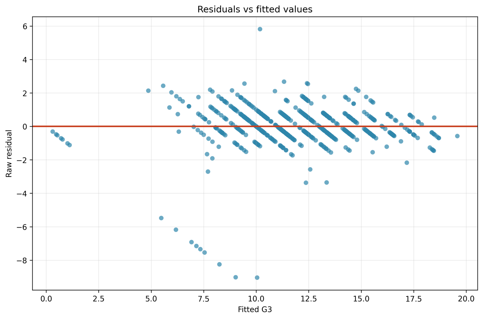
The scatter places raw residuals on the vertical axis and fitted G3 on the horizontal axis. Integer-valued grades create diagonal bands, but the changing vertical spread and several very negative errors are more important than the banding itself.
The fitted model uses 649 cases, has R² = 0.850632 and RMSE = 1.254409. Ramsey RESET = 10.774057 with p = 0.001085, while Breusch–Pagan p = 1.0237×10⁻⁵ and White p = 1.7529×10⁻⁶.
Regression Diagnostics separates mean-form concerns from variance concerns. The RESET result suggests that the six-predictor linear mean may omit curvature or interactions, while the variance tests indicate that one constant residual variance is doubtful.
Inspect partial-residual plots, test defensible nonlinear terms, and compare ordinary standard errors with HC3 robust standard errors. Retain the original model as the reference when reporting sensitivity results.
Python Chart 2: Normal Q–Q Plot
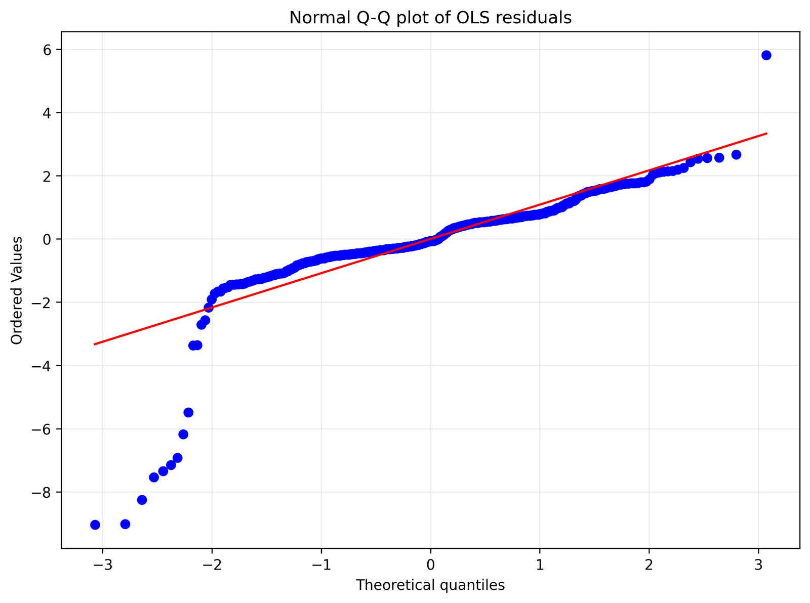
The middle residual quantiles follow the reference direction more closely than the tails. The lower tail bends sharply away because several observed grades of zero or one are predicted much higher by the model.
Shapiro–Wilk W = 0.754697 with p = 6.2445×10⁻³⁰. Jarque–Bera = 10152.729452 with p effectively below machine reporting precision. The maximum absolute externally studentized residual is 7.590715.
With 649 observations, formal normality tests are sensitive, but the conclusion is not based on p-values alone: the visible tail departures and the extreme deleted residuals are large enough to matter for conventional small-sample inference.
Report robust confidence intervals, review the boundary cases, and compare coefficient conclusions after verified-error corrections and influence sensitivity analysis. Do not delete valid cases simply to straighten the Q–Q plot.
Python Chart 3: Residual Histogram
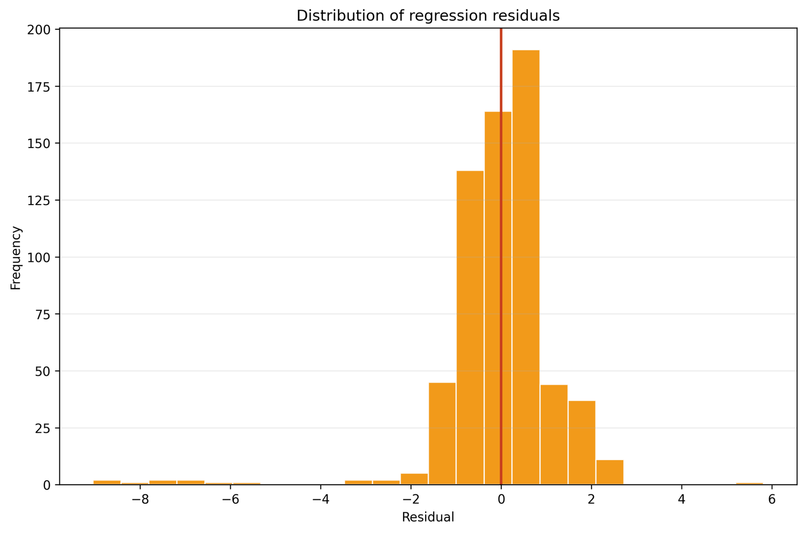
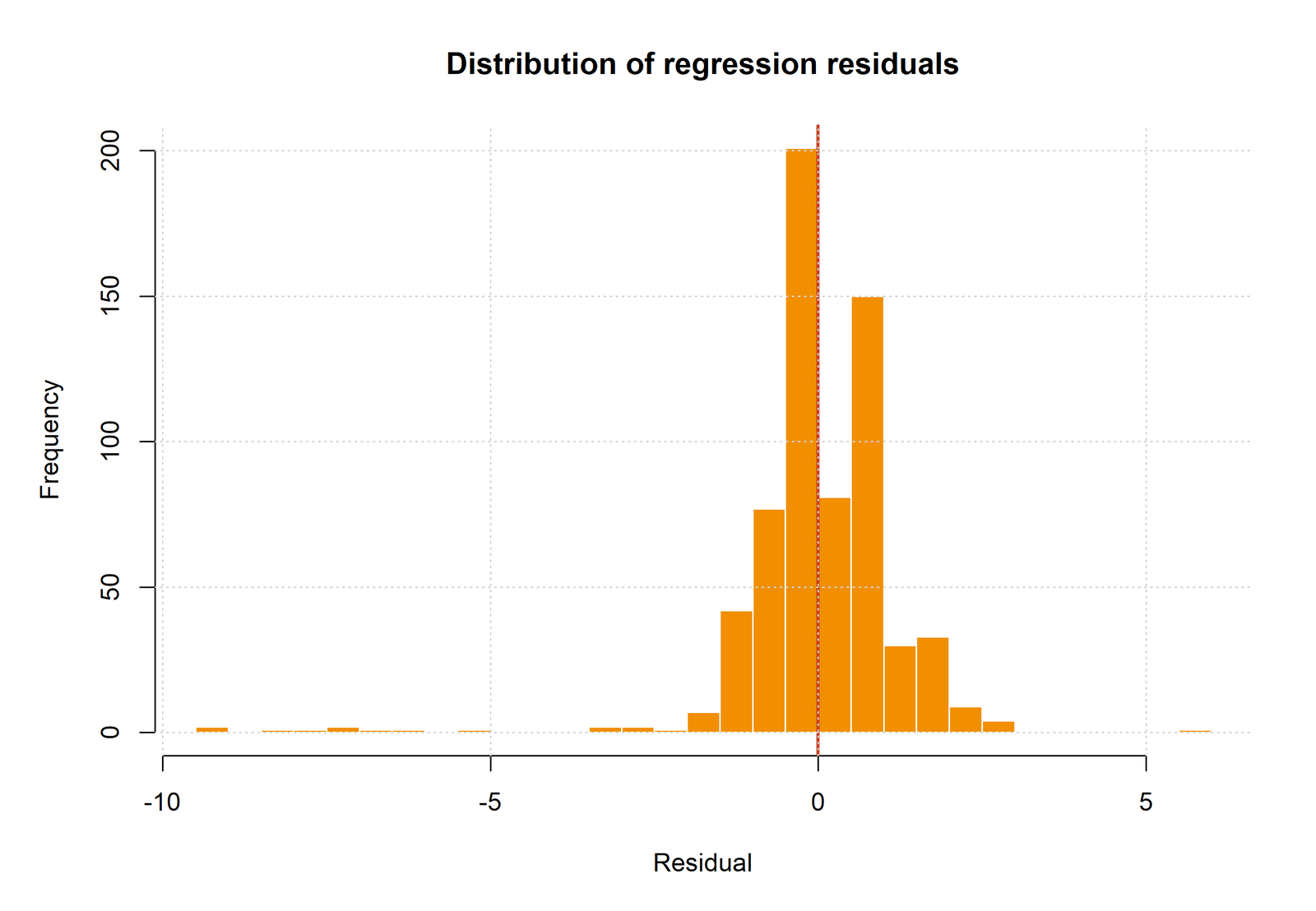
The histogram has a dense center near zero with a pronounced negative tail and a thinner positive tail. The central concentration explains why overall RMSE remains moderate even though a few cases have severe errors.
Ten observations exceed |externally studentized residual| > 3. Case 164 reaches −7.590715, case 173 reaches −7.545231, and case 62 reaches +4.727414.
Regression Diagnostics uses the histogram to summarize shape, but it cannot show which predictor profiles create the tail. The histogram therefore complements, rather than replaces, leverage and deletion-influence measures.
Identify whether the extreme low outcomes are coding errors, structural zeros, censored values, or valid members of the target population. Then repeat the model with documented alternatives rather than silently trimming the tails.
Python Chart 4: Scale–Location Plot
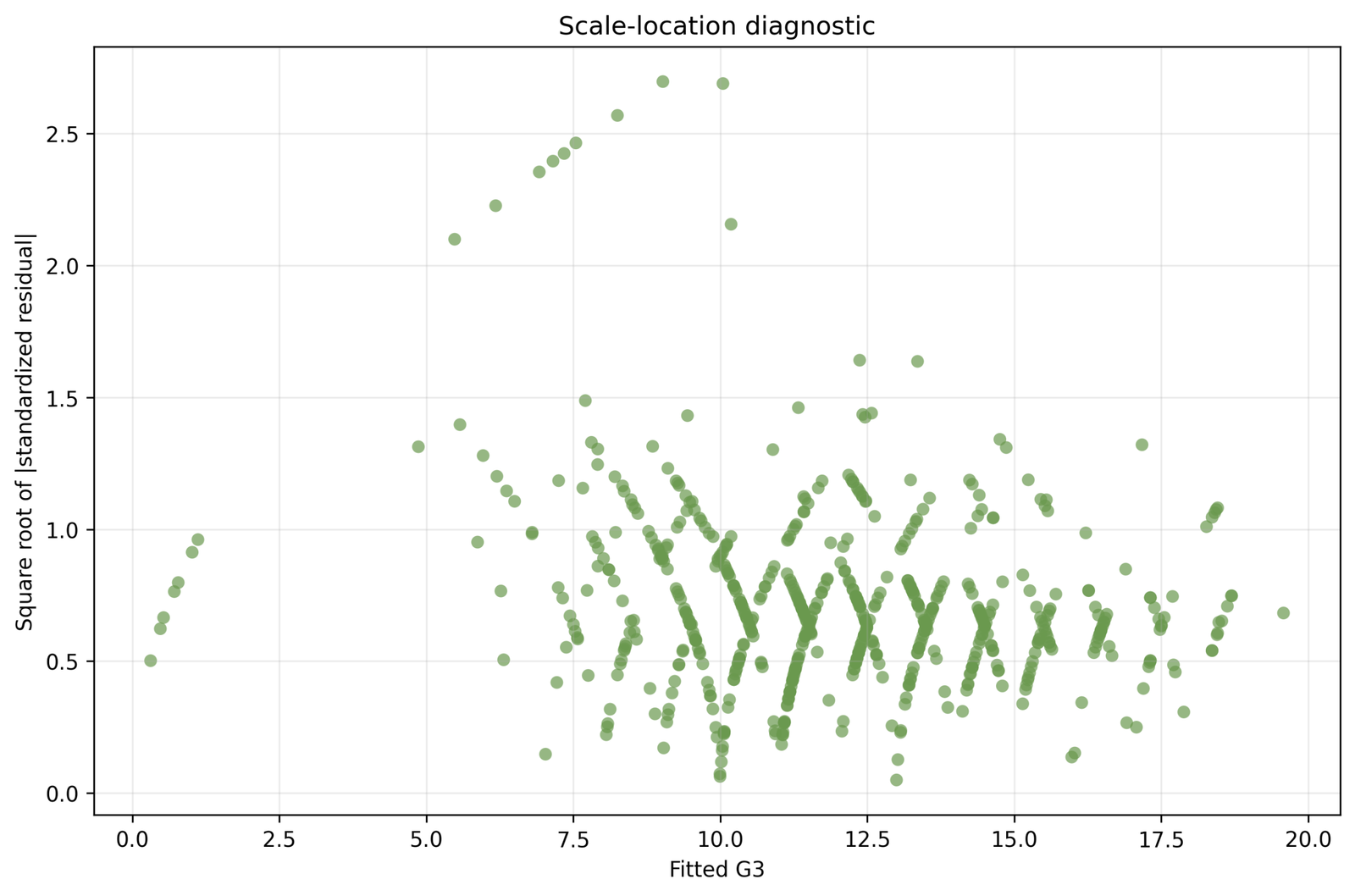
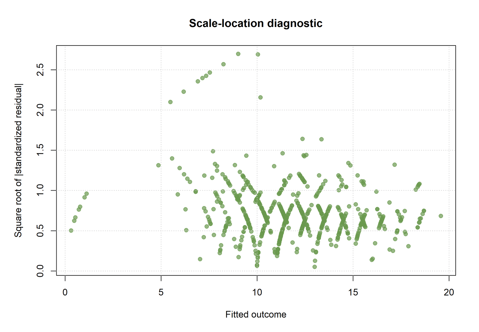
The square-root absolute standardized residuals do not form a perfectly horizontal band. Larger fitted values and boundary regions show different residual spread, which is consistent with nonconstant variance.
Breusch–Pagan LM = 33.054192, p = 1.0237×10⁻⁵. White LM = 75.547435, p = 1.7529×10⁻⁶. These tests agree with the visual concern.
Heteroscedasticity changes the reliability of ordinary OLS standard errors even when coefficient point estimates remain unbiased under an otherwise correct conditional-mean model. Regression Diagnostics therefore qualifies inferential claims, not only prediction error.
Calculate HC3 or another defensible heteroscedasticity-consistent covariance estimate, compare interval widths, and consider whether variance changes are linked to grade level, failures, absences, or the lower outcome boundary.
Python Chart 5: Studentized Residuals Versus Leverage
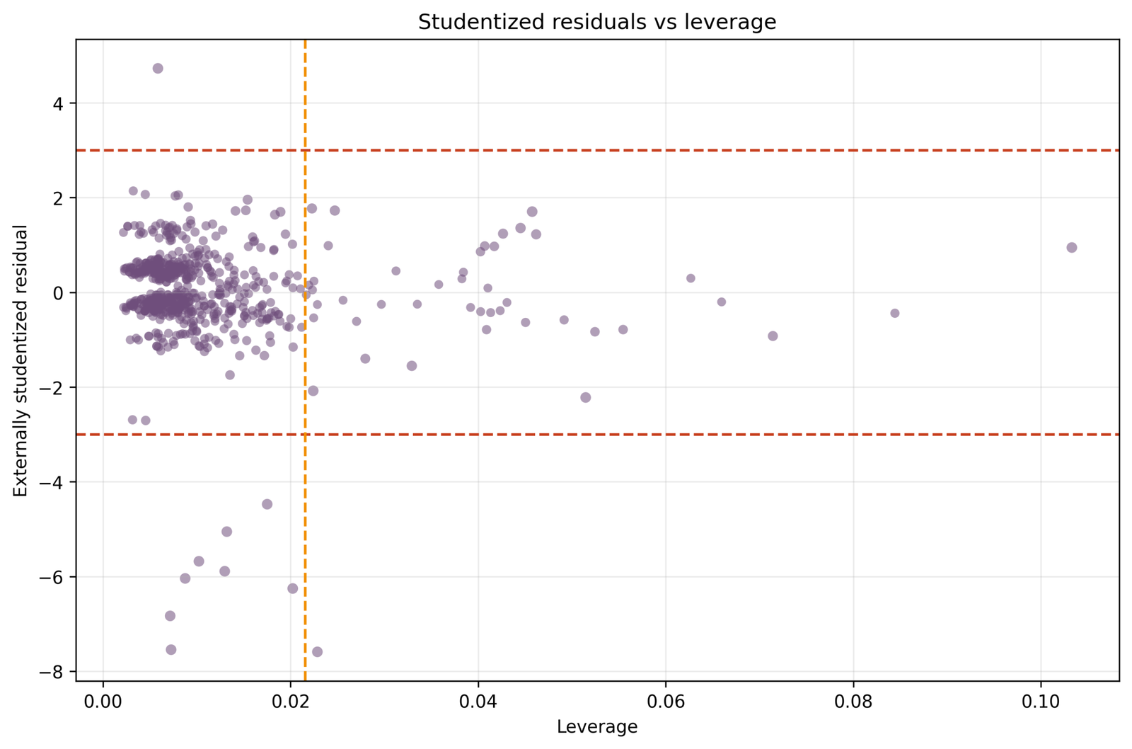
This joint plot distinguishes response outliers from unusual predictor combinations. Case 164 combines an extreme deleted residual with leverage just above the screening rule, whereas case 1 occupies the far-right leverage region with only a modest residual.
The leverage cutoff is 0.021572 and the residual cutoff is |3|. Case 164 has rstudent = −7.590715 and leverage = 0.022859. Case 1 has leverage = 0.103309 but rstudent = 0.944918.
High leverage is not equivalent to a bad observation. Regression Diagnostics asks whether a strategic predictor-space position is also associated with a large conditional error or a material deletion effect.
Review cases 164 and 1 for different reasons. For case 164, investigate the observed outcome and deletion sensitivity. For case 1, verify its predictor profile and compare the model with and without that high-leverage but non-outlying case.
Python Chart 6: Cook’s Distance by Case
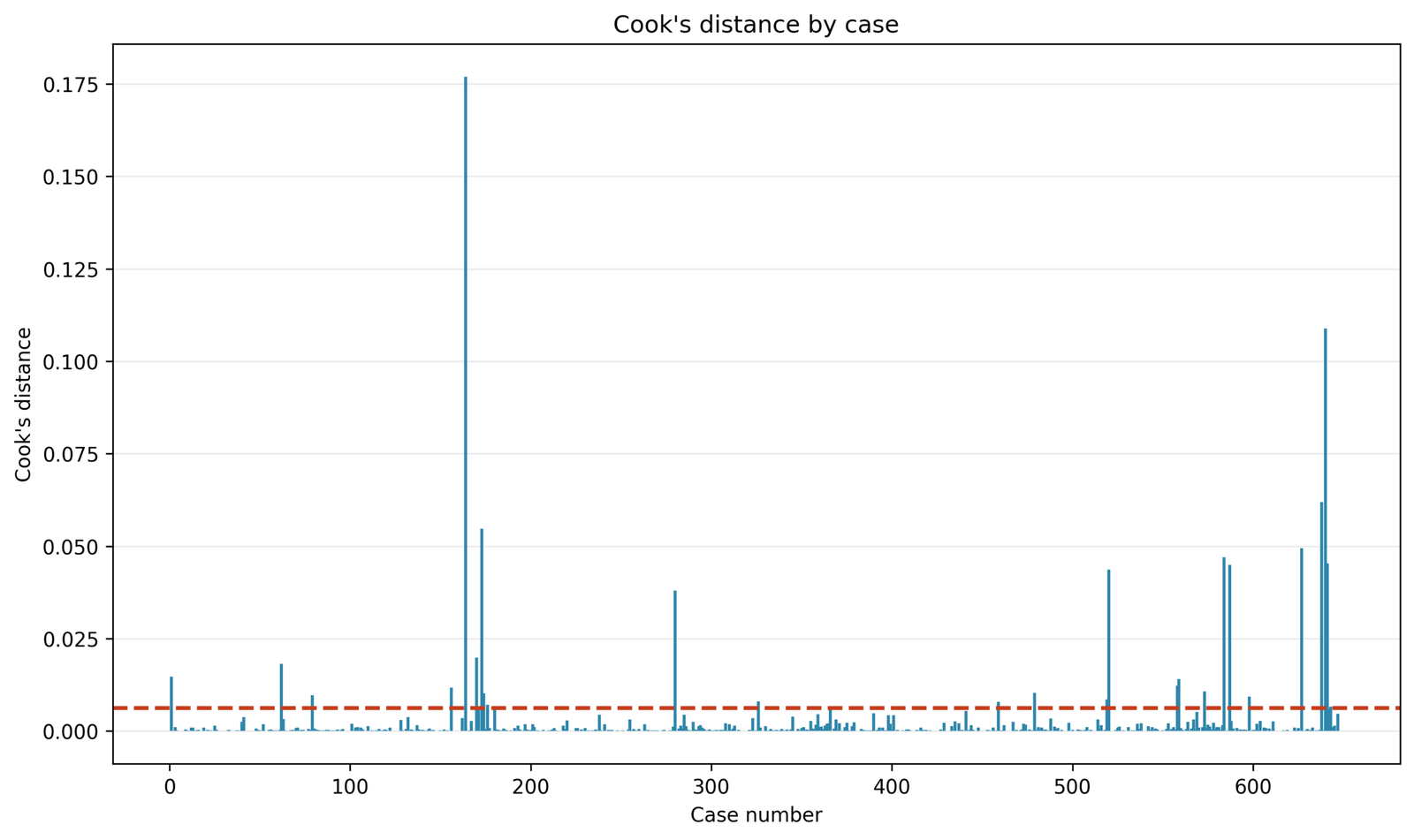
The sequence is dominated by a small number of spikes. Most cases have Cook’s distance near zero, while a compact influential set rises above the 4/n reference line.
The Cook’s distance cutoff is 0.006163. Twenty-six cases exceed it. The maximum is case 164 at 0.176952, followed by case 640 at 0.108871 and case 638 at 0.061908.
Cook’s distance summarizes how case deletion changes the fitted coefficient vector relative to its estimated covariance. It is a magnitude screen, not a significance test and not an automatic deletion command.
Refit the model after removing one case at a time for the leading observations, then compare coefficients, predicted values, R², robust intervals, and substantive conclusions. Record why each case is retained or excluded.
Python Chart 7: Observed Versus Predicted G3
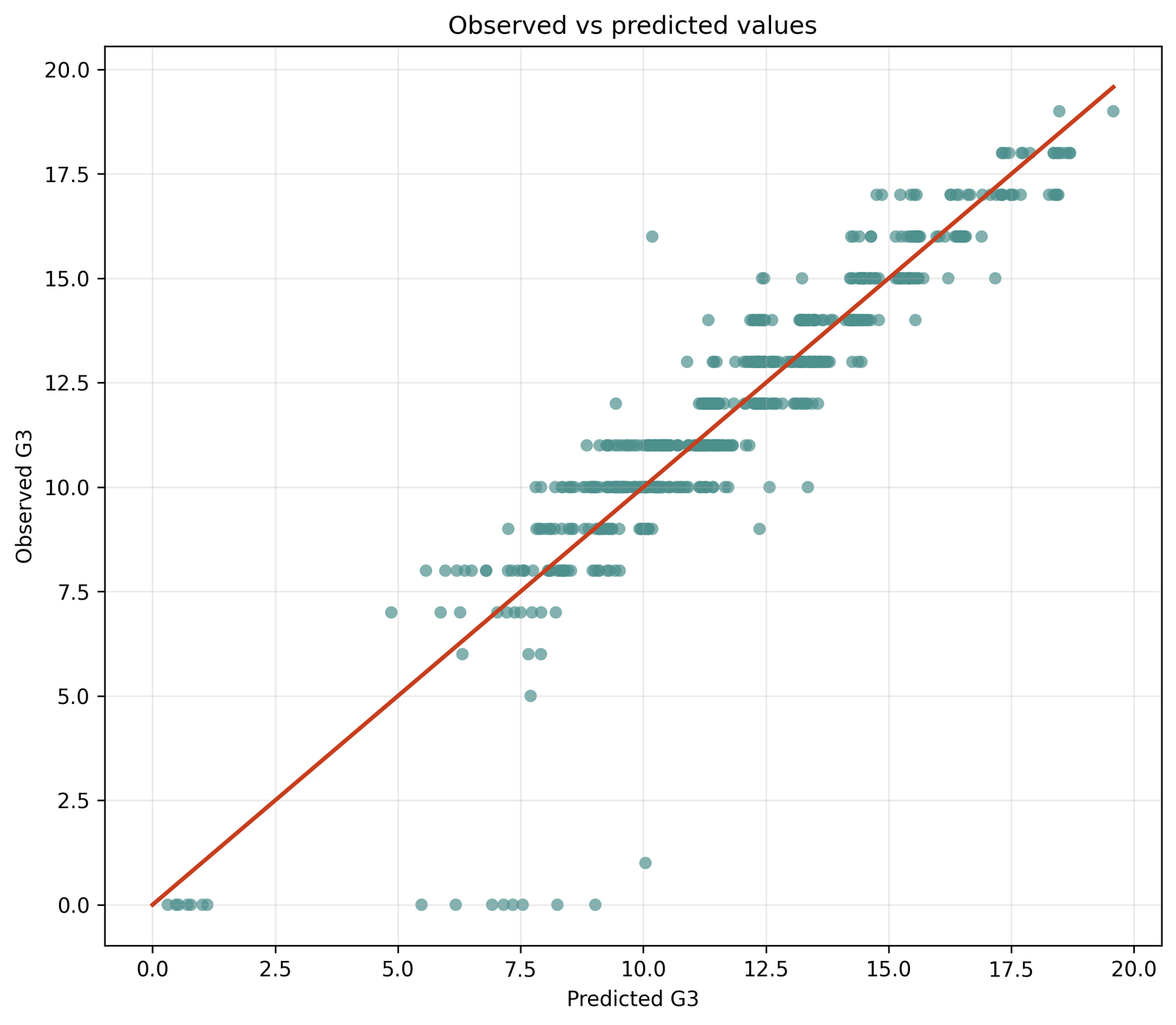
Most points track the diagonal through the central grade range, explaining the high fitted R². The largest departures occur at the lower boundary, where several observed zeros receive predictions between roughly five and ten.
R² = 0.850632, adjusted R² = 0.849236, and RMSE = 1.254409. Case 164 has G3 = 0 but predicted G3 = 9.022936; case 173 has G3 = 1 but predicted G3 = 10.044619.
Strong aggregate fit can coexist with systematic failure for a small but important outcome region. Regression Diagnostics therefore interprets the diagonal cloud together with tail, variance, and influence evidence.
Calculate subgroup error for zero and low grades, consider whether the outcome boundary requires a different model form, and compare out-of-sample performance before claiming general predictive accuracy.
Python Chart 8: Standardized Residuals by Case
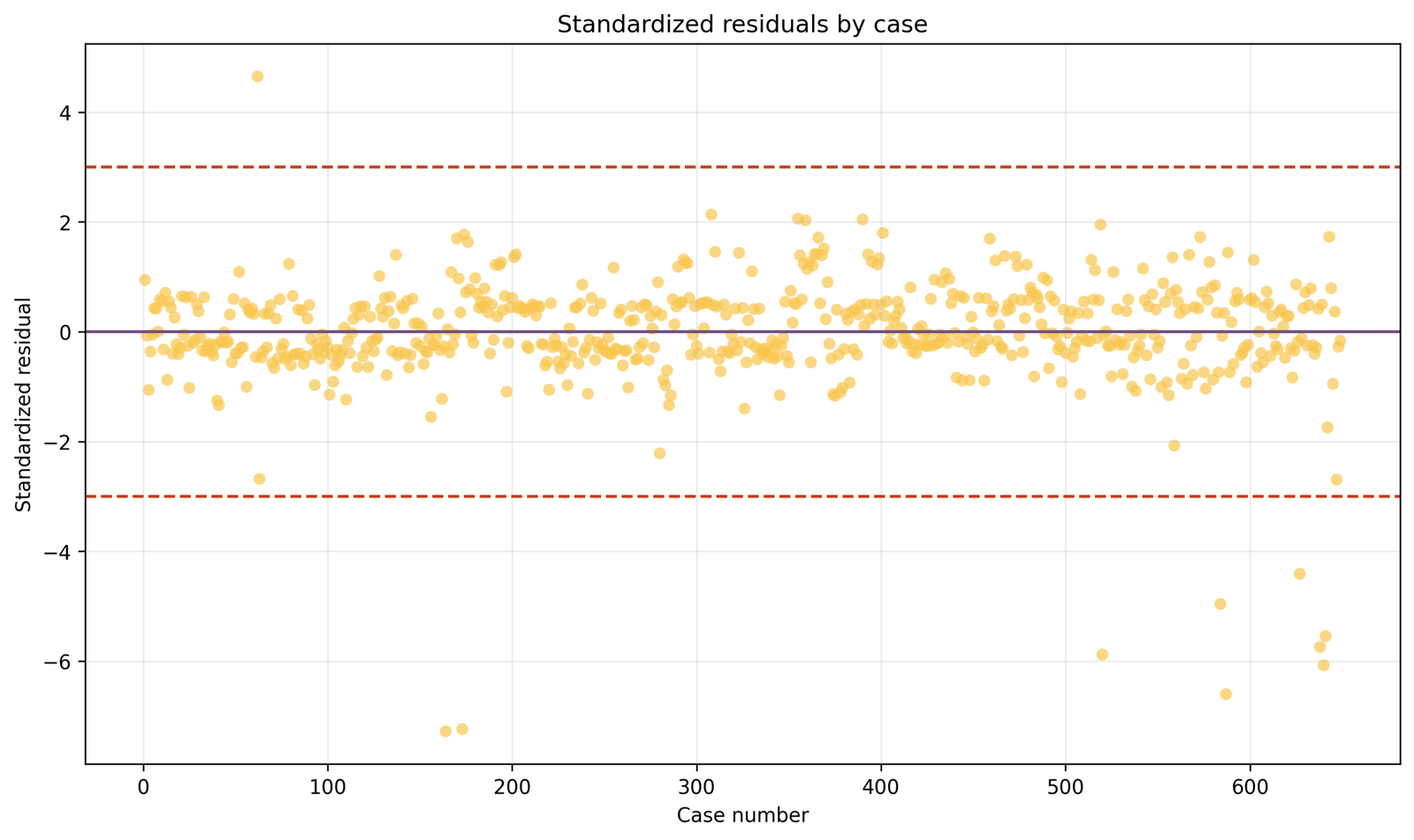
The sequence plot exposes isolated extremes and any order-related clustering that a histogram hides. Most standardized residuals remain near zero, but a small set of negative spikes dominates the range.
Ten cases exceed the deleted-residual rule of |3|. Durbin–Watson = 1.860956, which is near 2, although its meaning depends on whether row order has a substantive temporal or spatial interpretation.
Regression Diagnostics should not treat a near-2 Durbin–Watson value as proof of independence in cross-sectional data. Independence is primarily a design assumption; the sequence is useful for discovering ordering artifacts or batches.
Verify how the data were ordered, check for school, class, family, or repeated-measure clustering, and use clustered or multilevel methods if observations are not independent units.
Python Chart 9: Leverage Versus Absolute DFFITS
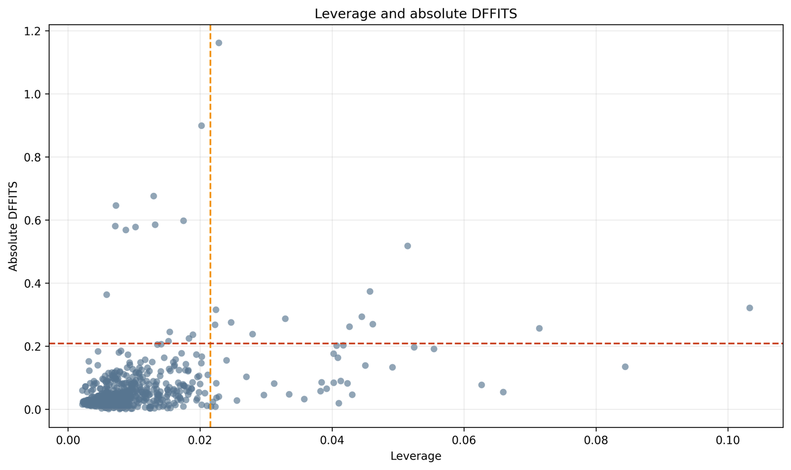
The plot separates unusual predictor geometry on the horizontal axis from fitted-value sensitivity on the vertical axis. Some observations cross both rules, while others are flagged by only one dimension.
The leverage rule is 0.021572 and the |DFFITS| rule is 0.207710. Forty-five cases exceed the leverage rule and twenty-six exceed the DFFITS rule. Maximum leverage is 0.103309; maximum |DFFITS| is 1.160994.
DFFITS asks how much the fitted value for a case changes after that case is deleted. Regression Diagnostics uses it alongside Cook’s distance because the two measures summarize related but not identical deletion effects.
Prioritize observations beyond both lines, then inspect cases beyond only one line. High-leverage cases with moderate DFFITS may still be valid anchors, while large DFFITS at modest leverage can reflect severe response mismatch.
Python Chart 10: Coefficient Confidence Intervals
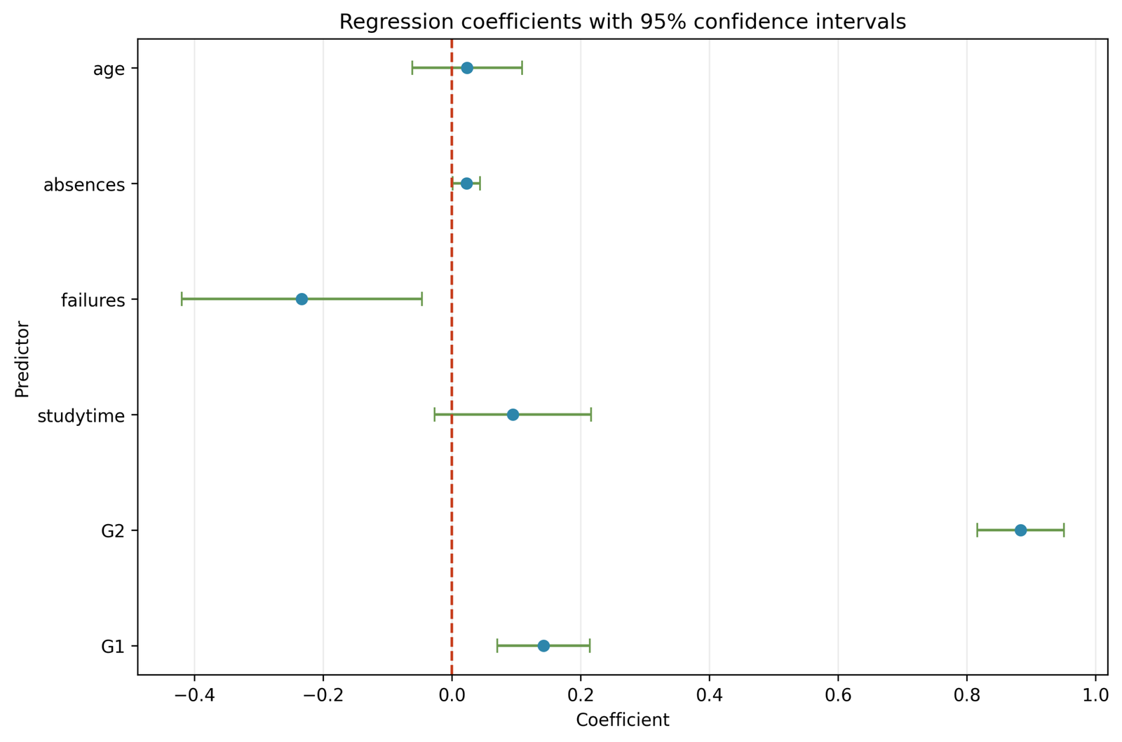
The interval plot presents the intercept and six predictor slopes from the original OLS model. It shows direction and uncertainty before any heteroscedasticity correction or influence sensitivity refit.
The model uses G1, G2, studytime, failures, absences, and age. VIF values range from 1.048621 to 4.154857, so the largest coefficient-overlap concern is the G1–G2 pair rather than a severe whole-model collinearity failure.
Because RESET, normality, and variance checks are significant, ordinary intervals should be treated as the starting specification. Regression Diagnostics does not invalidate every coefficient; it asks whether signs, magnitudes, and decisions survive better uncertainty estimates and plausible model changes.
Compare the displayed intervals with HC3 intervals, a nonlinear specification, and influence sensitivity refits. Report any coefficient whose sign or substantive interpretation depends on a small set of valid influential cases.
R Charts and Explanations
The supplied material contains four R diagnostic images and an R source excerpt, but it does not provide a completed downloadable R report PDF. The R section therefore interprets the visible reproductions against the verified model values without claiming a separate R-report audit that is not available.
rstandard(), rstudent(), hatvalues(), cooks.distance(), dffits(), and covratio(). A valid reproduction must preserve the same 649 complete cases, formula, and case numbering.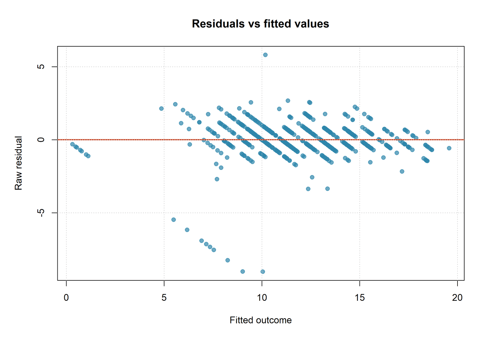
R Chart 1: Residuals Versus Fitted
The R display should show the same diagonal grade bands, lower-tail errors, and changing spread as the Python chart because it uses the same six-predictor equation and complete cases. The relevant numeric anchors remain R² = 0.850632, RESET p = 0.001085, Breusch–Pagan p = 1.0237×10⁻⁵, and White p = 1.7529×10⁻⁶.
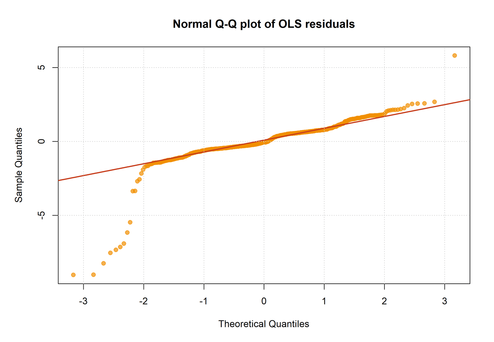
plot(model, which = 1) as a visual screen, then report formal mean-form and variance checks separately.R Chart 2: Normal Q–Q Plot
The lower and upper quantiles should depart from the straight reference line, with the lower tail showing the strongest problem. This agrees with Shapiro–Wilk W = 0.754697, p < .001, and the extreme externally studentized residuals.
R Chart 3: Residual Histogram
The histogram summarizes a strong central mass and a long negative tail created largely by unexpectedly low G3 outcomes. Ten deleted residuals exceed the absolute rule of three, so a normal-looking center must not obscure the influential tails.
hist(resid(model)) with rstudent(model), Cook’s distance, and case-level verification.R Chart 4: Scale–Location Plot
The spread of square-root absolute standardized residuals changes across fitted values. The pattern is consistent with both heteroscedasticity tests, so ordinary OLS standard errors should be compared with a robust covariance estimate.
Regression Diagnostics Parameter Interpretation
The word “outlier” is too broad for a complete Regression Diagnostics report. Each measure answers a different counterfactual question. The exact value and the case profile should be reported together.
| Measure | Observed maximum or range | What it means | Worked example |
|---|---|---|---|
| Externally studentized residual | Maximum absolute = 7.590715 | How surprising the outcome is after leverage and deleted-case scale adjustment. | Case 164 is far below its predicted grade. |
| Leverage | Maximum = 0.103309 | How unusual the predictor combination is relative to the design center. | Case 1 has the greatest predictor-space extremity. |
| Cook’s distance | Maximum = 0.176952 | Overall coefficient-vector change under one-case deletion. | Case 164 is the strongest deletion influence. |
| DFFITS | Maximum absolute = 1.160994 | Change in the case’s fitted value after deleting that case. | Case 164 again has the largest fitted-value sensitivity. |
| COVRATIO | Leading range 0.561339 to 1.116514 | Change in generalized coefficient covariance under deletion. | Case 173 sharply reduces covariance volume when deleted; case 1 increases it. |
| VIF | 1.048621 to 4.154857 | Inflation of slope variance due to predictor overlap. | G1 and G2 account for the main collinearity concern. |
Three Contrasting Case Profiles
Case 164: residual + leverage + influence
- G3 = 0; predicted = 9.022936
- rstudent = −7.590715
- leverage = 0.022859
- Cook’s D = 0.176952
- DFFITS = −1.160994
- COVRATIO = 0.566377
Case 1: leverage without severe residual
- G3 = 11; predicted = 9.877488
- rstudent = 0.944918
- leverage = 0.103309
- Cook’s D = 0.014698
- DFFITS = 0.320731
- COVRATIO = 1.116514
A total flag count is useful for sorting, but the units are incomparable. One residual flag and one COVRATIO flag do not represent equal increments of severity. Regression Diagnostics should describe the pathway: outcome surprise, predictor extremity, coefficient movement, fitted-value movement, or covariance movement.
Predictions, Influence and Model Meaning
The fitted equation predicts a continuous conditional mean for G3. Its R² of 0.850632 means that the six predictors explain about 85.06% of fitted-sample outcome variation under this model. It does not mean that every observation is predicted accurately, that residual assumptions are satisfied, or that the slopes are causal.
The observed-versus-predicted chart and the leading case table reveal a boundary problem. Several students with G3 = 0 have predictions above five, and the strongest case is predicted above nine. A linear mean can produce such errors when the outcome distribution has a mass at zero, a censoring mechanism, a special failure process, or predictor information not captured by the equation.
Regression Diagnostics Sensitivity Sequence
Check source values, units, duplicate rows, missing-value codes, and eligibility.
Use robust covariance, nonlinear terms, interactions, or a boundary-aware model.
Report which coefficients, intervals, and predictions remain stable.
Single-case sensitivity
- Delete case 164 and refit.
- Repeat for cases 640, 638, 173, and case 1.
- Compare slope changes and fitted values.
- Record whether signs or decisions change.
Grouped sensitivity
- Refit without verified errors only.
- Refit without all G3 = 0 cases as a sensitivity analysis, not a preferred model.
- Refit without the 62-case flagged union.
- Use bootstrap or cross-validation to assess stability.
Deleting all flagged cases is not automatically defensible. It may redefine the population by excluding precisely the students the model predicts poorly. The correct Regression Diagnostics report keeps the full-sample model visible and labels every restricted analysis as sensitivity evidence.
Regression Diagnostics Assumptions and Decisions
Evidence that is comparatively reassuring
- Overall fitted alignment is strong in the central grade range.
- Adjusted R² remains close to R².
- Scaled condition number is only 4.250230.
- Four VIF values are close to 1.
- Durbin–Watson is near 2, subject to meaningful ordering.
- Most cases have small Cook’s distance and DFFITS.
Evidence requiring action
- RESET rejects a simple linear functional form.
- Both variance tests reject homoscedasticity.
- Q–Q and histogram tails are severe.
- Ten deleted residuals exceed |3|.
- Case 164 has unusually broad influence.
- Lower-boundary G3 values are systematically difficult.
Functional Form
Ramsey RESET = 10.774057 with p = 0.001085 suggests that powers of the fitted values add information not represented by the original linear equation. This does not identify the correct term. A defensible next step is to inspect nonlinear effects of G1, G2, failures, absences, and age, plus interactions justified before examining the result.
Heteroscedasticity
Breusch–Pagan and White tests both reject constant variance. Regression Diagnostics should therefore compare ordinary and HC3 confidence intervals. Weighted least squares is appropriate only when a credible variance model is developed; it should not be applied solely because a test is significant.
Residual Normality
The sample is large enough that Shapiro–Wilk and Jarque–Bera can detect modest departures, but these departures are not modest. The Q–Q plot, histogram, and externally studentized residuals show a pronounced lower tail. Robust or bootstrap inference is preferable to pretending the residuals are normal.
Independence
Durbin–Watson = 1.860956 is near the conventional reference of 2. However, independence comes from design. If students are clustered within schools, classes, families, or repeated records, a cluster-robust or multilevel analysis may be needed even when the residual sequence appears acceptable.
Collinearity
G1 and G2 have VIF values just above 4. Their separate slopes may therefore be more sensitive than the other slopes, but the scaled condition number and remaining VIF values do not indicate a severe numerical breakdown. Centering does not remove overlap between G1 and G2; it mainly changes intercept interpretation.
Masking, Swamping and Multiple Influence
One-case diagnostics can mask a group of jointly influential observations or flag observations that cease to be important after another case is removed. A high-quality Regression Diagnostics workflow supplements one-row deletion with grouped deletion, bootstrap stability, and cross-validation.
Regression Diagnostics in Python, R, SPSS and Excel
Python
statsmodels provides fitted values, residuals, leverage, Cook’s distance, DFFITS, COVRATIO, VIF, and formal diagnostic tests. Python is the primary machine-readable workflow in this casebook.
- Use one complete-case dataframe.
- Preserve a separate case number.
- Save every diagnostic value and Boolean flag.
- Export plots, CSV tables, TXT narrative, and PDF report.
R
Base R provides the central casewise diagnostics through rstudent, hatvalues, cooks.distance, dffits, and covratio. Additional packages provide RESET, heteroscedasticity, and VIF checks.
- Use the same formula and rows as Python.
- Save case numbering before sorting.
- Compare leading values, not only plots.
- No completed R PDF download was supplied.
SPSS
SPSS REGRESSION can save predicted values, residual variants, Cook’s distance, leverage, and COVRATIO while producing casewise and collinearity output.
- Use the exact six-predictor equation.
- Set the outlier casewise threshold to 3.
- Save SPV and export a compatibility-safe PDF.
- Reconcile SPSS variable names with the audit workbook.
Excel
The worked workbook makes threshold arithmetic and Boolean logic transparent. It is best used to audit values generated by statistical software rather than to recreate every matrix calculation manually.
- Store n, k, and p explicitly.
- Lock threshold cells with absolute references.
- Count overlapping flags row by row.
- Sort on exact Cook’s D or flag count without losing case numbers.
Software outputs can differ when residual definitions, intercept handling, missing-data filters, or case numbering differ. Regression Diagnostics cross-software validation therefore begins with the same formula and data matrix, not with visual similarity alone.
Code: Expand Only the Software You Need
Python Regression Diagnostics workflow
from pathlib import Path
import math
import numpy as np
import pandas as pd
import statsmodels.api as sm
from scipy import stats
from statsmodels.stats.diagnostic import (
    het_breuschpagan, het_white, linear_reset
)
from statsmodels.stats.outliers_influence import (
    OLSInfluence, variance_inflation_factor
)
from statsmodels.stats.stattools import durbin_watson, jarque_bera

BASE_DIR = Path(r"D:\DATA ANALYSIS\H Regression Tests and Models\Regression Diagnostics")
df = pd.read_csv(BASE_DIR / "dataset.csv")
outcome = "G3"
predictors = ["G1", "G2", "studytime", "failures", "absences", "age"]
analysis = df[[outcome] + predictors].apply(pd.to_numeric, errors="coerce").dropna()

y = analysis[outcome].astype(float)
X = sm.add_constant(analysis[predictors].astype(float), has_constant="add")
model = sm.OLS(y, X).fit()
influence = OLSInfluence(model)

n = int(model.nobs)
k = len(predictors)
p = k + 1
fitted = np.asarray(model.fittedvalues)
raw_residual = np.asarray(model.resid)
internal_studentized = np.asarray(influence.resid_studentized_internal)
external_studentized = np.asarray(influence.resid_studentized_external)
leverage = np.asarray(influence.hat_matrix_diag)
cooks_d = np.asarray(influence.cooks_distance[0])
dffits = np.asarray(influence.dffits[0])
covratio = np.asarray(influence.cov_ratio)

thresholds = {
    "residual": 3.0,
    "leverage": 2.0 * p / n,
    "cooks_d": 4.0 / n,
    "dffits": 2.0 * math.sqrt(p / n),
    "covratio_lower": 1.0 - 3.0 * p / n,
    "covratio_upper": 1.0 + 3.0 * p / n,
}

case_table = analysis.reset_index(drop=False).rename(columns={"index": "source_case"})
case_table["case_number"] = np.arange(1, n + 1)
case_table["predicted"] = fitted
case_table["raw_residual"] = raw_residual
case_table["standardized_residual"] = internal_studentized
case_table["externally_studentized_residual"] = external_studentized
case_table["leverage"] = leverage
case_table["cooks_distance"] = cooks_d
case_table["dffits"] = dffits
case_table["covratio"] = covratio
case_table["residual_outlier_flag"] = np.abs(external_studentized) > thresholds["residual"]
case_table["high_leverage_flag"] = leverage > thresholds["leverage"]
case_table["high_cooks_flag"] = cooks_d > thresholds["cooks_d"]
case_table["high_dffits_flag"] = np.abs(dffits) > thresholds["dffits"]
case_table["covratio_flag"] = (
    (covratio < thresholds["covratio_lower"]) |
    (covratio > thresholds["covratio_upper"])
)
flag_columns = [
    "residual_outlier_flag", "high_leverage_flag", "high_cooks_flag",
    "high_dffits_flag", "covratio_flag"
]
case_table["number_of_flags"] = case_table[flag_columns].sum(axis=1)
case_table["any_diagnostic_flag"] = case_table["number_of_flags"] > 0

reset = linear_reset(model, power=2, use_f=True)
shapiro_w, shapiro_p = stats.shapiro(raw_residual)
jb_stat, jb_p, skew, kurtosis = jarque_bera(raw_residual)
bp_lm, bp_p, bp_f, bp_f_p = het_breuschpagan(raw_residual, X)
white_lm, white_p, white_f, white_f_p = het_white(raw_residual, X)
dw = durbin_watson(raw_residual)

vif = pd.DataFrame({
    "predictor": predictors,
    "vif": [variance_inflation_factor(analysis[predictors].values, i)
            for i in range(len(predictors))]
})
vif["tolerance"] = 1.0 / vif["vif"]

case_table.to_csv(BASE_DIR / "Python_Output/csv/regression_diagnostic_cases.csv", index=False)
print(model.summary())
print(thresholds)
print(reset, shapiro_w, shapiro_p, jb_stat, jb_p, bp_lm, bp_p, white_lm, white_p, dw)
R Regression Diagnostics workflow
base_dir <- "D:/DATA ANALYSIS/H Regression Tests and Models/Regression Diagnostics"
df <- read.csv(file.path(base_dir, "dataset.csv"), check.names = FALSE)
outcome <- "G3"
predictors <- c("G1", "G2", "studytime", "failures", "absences", "age")
analysis <- na.omit(df[c(outcome, predictors)])

formula_text <- paste(outcome, "~", paste(predictors, collapse = " + "))
model <- lm(as.formula(formula_text), data = analysis)

n <- nobs(model)
k <- length(predictors)
p <- k + 1
case_table <- data.frame(
  case_number = seq_len(n),
  analysis,
  predicted = fitted(model),
  raw_residual = resid(model),
  standardized_residual = rstandard(model),
  externally_studentized_residual = rstudent(model),
  leverage = hatvalues(model),
  cooks_distance = cooks.distance(model),
  dffits = dffits(model),
  covratio = covratio(model),
  check.names = FALSE
)

residual_cutoff <- 3
leverage_cutoff <- 2 * p / n
cook_cutoff <- 4 / n
dffits_cutoff <- 2 * sqrt(p / n)
covratio_lower <- 1 - 3 * p / n
covratio_upper <- 1 + 3 * p / n

case_table$residual_outlier_flag <- abs(case_table$externally_studentized_residual) > residual_cutoff
case_table$high_leverage_flag <- case_table$leverage > leverage_cutoff
case_table$high_cooks_flag <- case_table$cooks_distance > cook_cutoff
case_table$high_dffits_flag <- abs(case_table$dffits) > dffits_cutoff
case_table$covratio_flag <- case_table$covratio < covratio_lower |
                            case_table$covratio > covratio_upper
case_table$number_of_flags <- rowSums(case_table[c(
  "residual_outlier_flag", "high_leverage_flag", "high_cooks_flag",
  "high_dffits_flag", "covratio_flag"
)])
case_table$any_diagnostic_flag <- case_table$number_of_flags > 0

# Optional formal tests when packages are installed.
# lmtest::bptest(model)
# lmtest::resettest(model, power = 2, type = "fitted")
# car::vif(model)
# nortest::ad.test(resid(model))

write.csv(
  case_table,
  file.path(base_dir, "R_Output/tables/regression_diagnostic_cases.csv"),
  row.names = FALSE
)
summary(model)
SPSS Regression Diagnostics syntax
DATASET CLOSE ALL.
OUTPUT CLOSE ALL.
GET DATA
 /TYPE=TXT
 /FILE='D:\DATA ANALYSIS\H Regression Tests and Models\Regression Diagnostics\dataset.csv'
 /ENCODING='UTF8'
 /DELCASE=LINE
 /DELIMITERS=","
 /ARRANGEMENT=DELIMITED
 /FIRSTCASE=2
 /IMPORTCASE=ALL.
DATASET NAME RegressionDiagnostics.

REGRESSION
 /DEPENDENT G3
 /METHOD=ENTER G1 G2 studytime failures absences age
 /STATISTICS COEFF OUTS R ANOVA COLLIN TOL CI(95)
 /RESIDUALS HISTOGRAM(ZRESID) NORMPROB(ZRESID)
 /CASEWISE PLOT(ZRESID) OUTLIERS(3)
 /SAVE PRED RESID ZRESID SRESID SDRESID COOK LEVER COVRATIO.

* The saved variables support case review. DFFITS and exact threshold flags
* can be calculated in Python, R, or Excel when the installed SPSS release
* does not expose a directly saved DFFITS variable.

OUTPUT SAVE OUTFILE='D:\DATA ANALYSIS\H Regression Tests and Models\Regression Diagnostics\SPSS_Output\spv\Regression-Diagnostics-SPSS-Output.spv'.
OUTPUT EXPORT
 /CONTENTS EXPORT=ALL LAYERS=PRINTSETTING MODELVIEWS=PRINTSETTING
 /PDF DOCUMENTFILE='D:\DATA ANALYSIS\H Regression Tests and Models\Regression Diagnostics\SPSS_Output\pdf\Regression-Diagnostics-SPSS-Output.pdf'.
Excel Regression Diagnostics formulas
Assume:
B2 = n = 649
B3 = k = 6 predictors
B4 = p = k + 1 = 7 parameters including the intercept

Leverage cutoff:      =2*B4/B2
Cook's D cutoff:      =4/B2
DFFITS cutoff:        =2*SQRT(B4/B2)
COVRATIO lower:       =1-3*B4/B2
COVRATIO upper:       =1+3*B4/B2

Example row flags when the diagnostic values are in columns J:N:
Residual flag:        =ABS(J2)>3
Leverage flag:        =K2>$B$5
Cook flag:            =L2>$B$6
DFFITS flag:          =ABS(M2)>$B$7
COVRATIO flag:        =OR(N2<$B$8,N2>$B$9)
Number of flags:      =COUNTIF(O2:S2,TRUE)
Any diagnostic flag:  =T2>0
Advanced Regression Diagnostics Topics
Regression Diagnostics Analysis Map
- Fix the outcome, predictors, sample, and intercept.
- Fit and preserve the reference OLS model.
- Inspect residuals versus fitted values.
- Inspect residual shape and tail cases.
- Calculate leverage and deletion measures.
- Rank exact values and review case profiles.
- Run functional-form and variance checks.
- Compare ordinary and robust covariance estimates.
- Test defensible nonlinear or interaction terms.
- Perform one-case and grouped-case sensitivity.
- Assess out-of-sample prediction when relevant.
- Report stability and limitations transparently.
Why heuristic cutoffs are not significance tests
The 4/n Cook rule, 2p/n leverage rule, and 2√(p/n) DFFITS rule are convenient screens. They do not have a universal null distribution that turns every exceedance into a statistically significant problem. In a sample of 649, small cutoffs naturally produce many flags. Exact magnitude and conclusion change are more informative.
Masking and swamping
Masking occurs when several influential cases protect one another from appearing extreme in one-case diagnostics. Swamping occurs when ordinary cases appear influential because of other extreme observations. Group-deletion analysis and robust methods help reveal these patterns.
HC0, HC1, HC2 and HC3 robust covariance
HC estimators adjust coefficient covariance for heteroscedasticity. HC3 gives stronger leverage correction and is a common default for moderate samples. Robust covariance changes standard errors and intervals, not the OLS point estimates.
Robust regression is not automatic deletion
Huber or MM-estimation downweights observations according to a chosen loss function. It can be a useful sensitivity model, but it answers a different estimating question. Report both the reference OLS and the robust result.
Boundary-aware outcome models
G3 is bounded and contains zeros. A two-part process, censoring model, ordinal model, nonlinear mean, or separate structural explanation may fit the lower boundary better. The correct choice depends on how zero grades arise, not only on the residual plot.
DFBETAS and coefficient-specific influence
Cook’s distance summarizes global coefficient movement. DFBETAS identify which slope changes most after deletion. A case can have a moderate global Cook value but a large effect on one scientifically important coefficient.
Cross-validation after diagnostic revision
A revised equation should not be accepted merely because residual plots look cleaner in the fitted sample. Compare predictive error under repeated cross-validation or a held-out test set, with the entire transformation and selection process repeated inside each training split.
Regression Diagnostics Limitations
The current evidence is based on one six-predictor OLS specification. It does not prove that the strongest cases are incorrect, does not establish a causal structure, and does not identify the uniquely correct nonlinear alternative. The R images and code support reproduction, but no completed R report PDF is available. The SPSS and Excel files provide additional review, yet cross-software agreement still depends on identical rows and definitions.
APA-Style Reporting
An APA-style Regression Diagnostics paragraph should state the model, sample, fit, global diagnostic concerns, casewise influence, and planned sensitivity analysis. Avoid listing p-values without explaining how they qualify the interpretation.
When space is limited, report the most consequential evidence rather than every flagged count. The complete report can provide threshold definitions, full case tables, VIF values, and the leading observation profiles.
Publication Checklist
Model and data
- State G3 as the outcome.
- List all six predictors and the intercept.
- Report n = 649 complete cases.
- Explain any excluded rows or recoding.
- Preserve case numbering across outputs.
- Distinguish fitted from validation accuracy.
Regression Diagnostics evidence
- Report R², adjusted R², and RMSE.
- Define residual, leverage, Cook, DFFITS, and COVRATIO rules.
- Report overlapping flag counts correctly.
- Show exact leading case values.
- Reconcile every chart with the tables.
- Explain why a flag is not an automatic deletion.
Assumptions and inference
- Report RESET, variance, and residual-shape evidence.
- Explain whether row order makes Durbin–Watson meaningful.
- Report VIF and tolerance.
- Compare ordinary and robust covariance.
- Consider clustering or repeated observations.
- State the limits of causal interpretation.
Sensitivity and resources
- Verify high-priority records.
- Refit leading cases one at a time.
- Perform grouped-case sensitivity.
- Test only defensible alternative forms.
- Verify all report and chart links.
- Do not claim a missing R report download.
Downloads and Chart Resources
The verified downloadable evidence includes the Python PDF, the SPSS PDF, and the worked Excel workbook. Four R chart files and an R code excerpt are available on the page, but no completed R report PDF URL was supplied.
Regression Diagnostics Chart Files
Frequently Asked Questions
How many observations are flagged by Regression Diagnostics?
Sixty-two of 649 observations cross at least one prespecified residual, leverage, Cook, DFFITS, or COVRATIO screen. The individual category counts overlap and must not be added.
Which observation is most influential?
Case 164 has the largest Cook’s distance, 0.176952, and largest absolute DFFITS, 1.160994. It also has an externally studentized residual of −7.590715, leverage of 0.022859, and COVRATIO of 0.566377.
Is high leverage the same as a residual outlier?
No. High leverage describes an unusual predictor combination. A residual outlier has an unusual outcome given its predictors. Case 1 has maximum leverage but only a modest externally studentized residual.
Does Cook’s distance above 4/n prove a case is harmful?
No. The worked cutoff of 0.006163 is a screening convention. Practical concern depends on exact Cook magnitude, data validity, DFFITS, coefficient-specific influence, and changes in substantive conclusions.
Why are 45 leverage cases flagged?
The threshold 2p/n is small in a sample of 649. It is designed for triage. Many cases can exceed it without materially changing the regression, which is why leverage must be combined with residual and deletion measures.
What does COVRATIO measure?
COVRATIO measures the change in generalized coefficient covariance after deleting a case. Values below 0.967643 or above 1.032357 are screened in this analysis.
Do significant normality tests invalidate OLS?
They do not automatically invalidate coefficient point estimates, but they challenge conventional small-sample inference. Here the visible tail departures and extreme studentized residuals are also severe, so robust or bootstrap inference is warranted.
What should be done about heteroscedasticity?
Compare ordinary intervals with HC3 robust intervals, inspect whether spread changes with specific predictors or grade levels, and consider a defensible variance or outcome model. Do not use weighted least squares without a credible weight model.
Should all 62 flagged observations be deleted?
No. That would mechanically redefine the population and could bias the analysis. Verify errors, retain valid cases in the reference model, and label restricted refits as sensitivity analyses.
Why is there no R report download?
The supplied page contains R code and four R chart assets, but no completed R PDF report URL. The post therefore shows the reproducible R method and visuals without inventing a download.
Can Regression Diagnostics identify the correct nonlinear model?
No. RESET and residual plots indicate that the current form may be incomplete, but scientific knowledge and validation are required to choose transformations, interactions, or a different outcome family.
What is the main reporting conclusion?
The model has strong fitted-sample accuracy, but functional-form, heteroscedasticity, residual-tail, and influence evidence require robust uncertainty and documented sensitivity analysis before coefficient conclusions are treated as stable.
Regression Diagnostics Conclusion
Regression Diagnostics shows that the six-predictor G3 model is useful but not uniformly reliable. The central fitted relationship is strong, R² = 0.850632, yet RESET, Breusch–Pagan, White, Shapiro–Wilk, Jarque–Bera, the Q–Q plot, and the leading case profiles identify meaningful weaknesses. Sixty-two observations receive at least one screen, and case 164 has the greatest combined residual and deletion influence.
The correct response is not automatic case removal. Verify source records, keep the full-sample OLS result as the reference, compare HC3 uncertainty, examine defensible nonlinear or boundary-aware forms, perform one-case and grouped-case sensitivity, and report whether coefficient signs, intervals, and predictions remain stable. That sequence turns Regression Diagnostics from a collection of warning plots into an auditable model-quality decision process.

