Descriptive Statistics, Relative Variability and CV Percentage
Coefficient of Variation is a descriptive-statistics measure used to compare relative variability across variables, groups or measurement scales. This complete guide explains the coefficient of variation formula, CV percentage, interpretation rules, SPSS output, R workflow, Python workflow, Excel method and verified student-por.csv examples using G1, G2, G3, absences, school, sex, studytime and past-failure groups.
Google AdSense top placement reserved here
Quick Answer: Coefficient of Variation Result
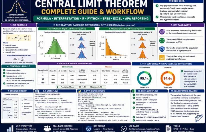
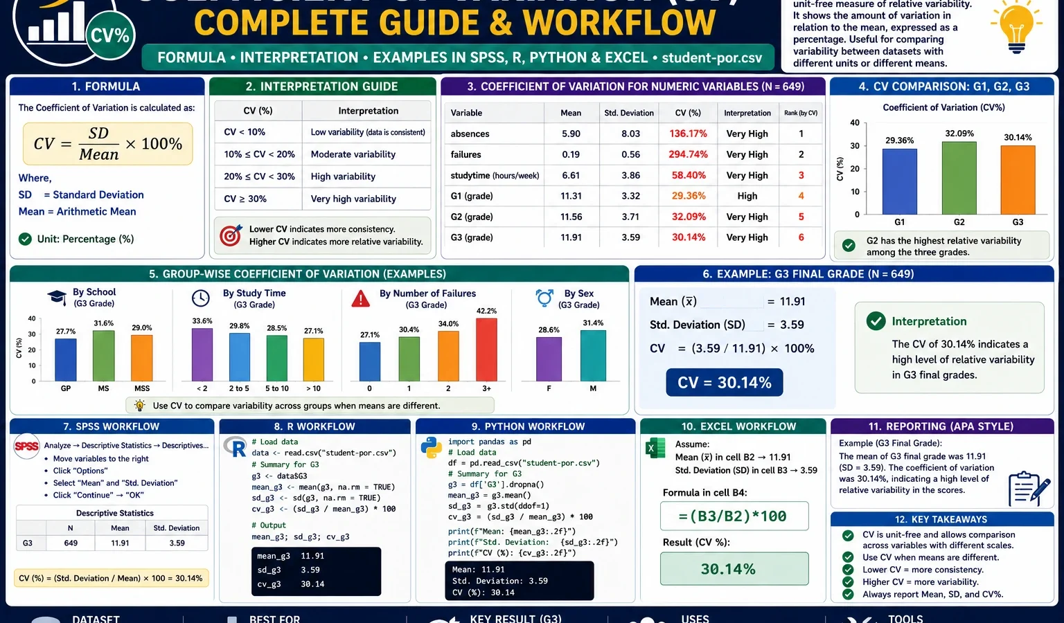
The Coefficient of Variation was calculated from the existing clean dataset file spss_ready_data.csv. The main formula used was CV% = (standard deviation / mean) × 100. For the grade variables, the CV values show that G3 final grade has slightly higher relative variability than G1 and G2, while absences has much higher relative variability because its standard deviation is larger than its mean.
Final report sentence: The coefficient of variation was used to compare relative variability across student performance variables. G1, G2 and G3 showed moderate relative variability, with G3 having the largest CV among the three grade measures. The absences variable showed the highest relative variability because absence counts are strongly spread relative to their mean. Therefore, CV is useful here because it compares variability in percentage form rather than using standard deviation alone.
Important reporting note: The coefficient of variation should be used carefully when the mean is zero, very close to zero or negative. In those cases, CV can become misleading or mathematically unstable.
Table of Contents
- What Is the Coefficient of Variation?
- Coefficient of Variation Formula
- Does Coefficient of Variation Have Hypotheses?
- Dataset and Existing Clean File Used
- Verified Results in SPSS, R and Python
- Python Charts and Interpretation
- R Validation Charts
- How to Calculate CV in SPSS, R, Python and Excel
- How to Report Coefficient of Variation
- Common Mistakes
- Download SPSS Output
- FAQs
What Is the Coefficient of Variation?
The Coefficient of Variation is a measure of relative variability. It compares the standard deviation of a variable with its mean. Instead of asking only how large the standard deviation is, CV asks how large the standard deviation is compared with the average value of the same variable.
This makes the coefficient of variation very useful when two variables are measured on different scales or when the means are very different. For example, a standard deviation of 3 may look small or large depending on whether the mean is 5, 50 or 500. CV solves this problem by expressing variability as a percentage of the mean.
In the student-por.csv dataset, the coefficient of variation helps compare the relative spread of grade variables such as G1, G2 and G3. It also shows why absences behaves very differently from grades. Grades have a clear range and a moderate spread, while absences have a low mean and a wide spread, so their CV becomes much larger.
Practical note: Standard deviation tells you the absolute spread. Coefficient of variation tells you the spread relative to the mean. That is why CV is often called relative standard deviation.
If you are learning descriptive statistics step by step, combine this guide with related Salar Cafe resources such as Box Plot Interpretation, Central Limit Theorem, Q-Q Plot Normality Check, Kolmogorov-Smirnov Test, DAgostino Pearson Test and Cramer von Mises Test.
Coefficient of Variation Formula
The basic Coefficient of Variation formula is:
Coefficient of Variation = Standard Deviation / MeanMost reports present the coefficient of variation as a percentage:
CV% = (Standard Deviation / Mean) × 100In symbols, the formula is:
CV% = (s / x̄) × 100Here, s is the sample standard deviation and x̄ is the sample mean. If the CV is 25%, it means the standard deviation is about one quarter of the mean. If the CV is 100%, it means the standard deviation is about equal to the mean.
| CV percentage | General meaning | Practical interpretation |
|---|---|---|
| Low CV | Values are relatively consistent around the mean. | The variable has low relative variability. |
| Moderate CV | Values show noticeable spread compared with the mean. | The variable has moderate relative variability. |
| High CV | The standard deviation is large compared with the mean. | The variable is highly variable relative to its average. |
| Very high CV | The mean may be small or the spread may be large. | Check the raw distribution before reporting the result. |
Does Coefficient of Variation Have a Null Hypothesis and Alternative Hypothesis?
The Coefficient of Variation is usually a descriptive statistic, not a hypothesis test. It does not automatically produce a p-value, null hypothesis or alternative hypothesis. It describes relative variability in a variable or group.
| Use case | Is it a hypothesis test? | What CV tells you |
|---|---|---|
| Compare G1, G2 and G3 variability | No | Which grade measure has more relative spread. |
| Compare G3 CV by school | No | Which school group has more relative grade variation. |
| Compare absences CV by failures group | No | Which failure group has more relative attendance variation. |
| Test whether two CVs differ significantly | Yes, but requires a special CV comparison test | This is beyond ordinary descriptive CV reporting. |
For a normal descriptive statistics report, write the mean, standard deviation and CV percentage. If you need formal inference, then use a specific statistical test designed for comparing coefficients of variation.
Google AdSense middle placement reserved here
Dataset and Existing Clean File Used
This worked example uses the existing clean file spss_ready_data.csv inside the Coefficient of Variation folder. No new cleaned dataset is needed for this article. The same existing clean file should be used for Python, R and SPSS so that all results match.
Important workflow rule: Use the existing spss_ready_data.csv file for all scripts. Do not create a different cleaned dataset when the clean file already exists in the folder.
| Item | Value used | Explanation |
|---|---|---|
| Topic folder | D:\DATA ANALYSIS\A Basic Descriptive Statistics Guides\Coefficient of Variation | Main output folder for this guide. |
| Clean data file | spss_ready_data.csv | Existing cleaned file used by R, Python and SPSS. |
| Main statistic | Coefficient of Variation | Relative variability measured as SD divided by mean. |
| Main variables | G1, G2, G3, absences | Used for numeric-variable CV comparison. |
| Grouping variables | school, sex, studytime, failures | Used for group-wise CV comparisons. |
| Sample size | 649 | Valid student records in the clean file. |
External dataset source: UCI Machine Learning Repository: Student Performance dataset.
Verified Results in SPSS, R and Python
The Coefficient of Variation workflow was reproduced in SPSS, R and Python using the same existing clean file. Python generated the publication charts, R generated validation charts, and SPSS produced the corrected output PDF for descriptive statistics and CV interpretation.
Main Grade Variable CV Results
The grade variables show moderate relative variability. The CV increases slightly from G1 to G3, meaning the final grade has a somewhat larger relative spread than the earlier grade measurements.
| Variable | Mean | Standard deviation | CV% | Interpretation |
|---|---|---|---|---|
| G1 | 11.3991 | 2.7453 | 24.08% | Moderate relative variability in first-period grade. |
| G2 | 11.5701 | 2.9136 | 25.18% | Moderate relative variability in second-period grade. |
| G3 | 11.9060 | 3.2307 | 27.13% | Highest relative variability among the three grade measures. |
Why Absences Has a Much Higher CV
The absences variable behaves differently from G1, G2 and G3. Its mean is low, but its standard deviation is large relative to that mean. This creates a high coefficient of variation and shows that absences are highly uneven across students.
| Variable | Mean | Standard deviation | CV% | Interpretation |
|---|---|---|---|---|
| absences | 3.6595 | 4.6408 | 126.82% | Very high relative variability; absence counts are strongly spread compared with their mean. |
SPSS Output Transcript
The corrected SPSS output confirms that the clean data file was imported properly and that coefficient of variation values were calculated from the correct mean and standard deviation values. The important transcript for reporting is: CV percentage was calculated as standard deviation divided by mean multiplied by 100. For grade variables, G3 had the highest CV among G1, G2 and G3. For attendance behavior, absences had the largest CV because the distribution is much more variable relative to its mean.
SPSS report sentence: Descriptive statistics showed that G1, G2 and G3 had moderate relative variability, while absences had very high relative variability. The coefficient of variation for G3 was about 27.13%, compared with about 24.08% for G1 and 25.18% for G2. The coefficient of variation for absences was much higher, about 126.82%, showing that absence counts varied strongly relative to their mean.
Python Charts and Interpretation
1. Coefficient of Variation for Numeric Variables

This chart compares CV values across the main numeric variables. It shows that variables with low means and large spread can have very high CV values. This is why absences appears much more variable than the grade variables when relative variability is used.
2. CV Comparison for G1, G2 and G3

This chart focuses on the three grade variables. The CV values are fairly close, but G3 is slightly higher. This means final grades are somewhat more variable relative to their mean than G1 and G2.
3. Mean, Standard Deviation and CV Scatter

This chart explains the logic behind the coefficient of variation. A variable can have a moderate standard deviation but still show a high CV if its mean is small. The chart helps readers see that CV is not just another name for standard deviation; it is standard deviation interpreted relative to the mean.
4. G3 Coefficient of Variation by School

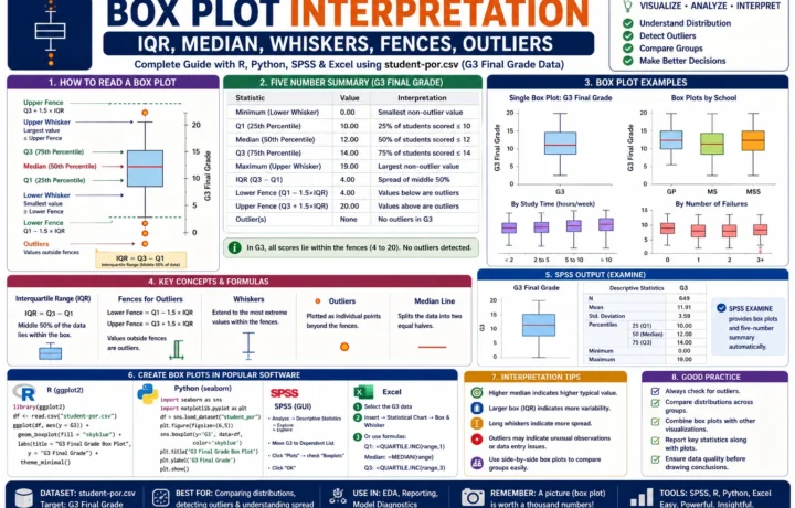
This chart compares the relative variability of G3 final grades across school groups. Group-wise CV is useful because two schools may have similar mean performance but different spread. A higher group CV means grades are less consistent within that group.
5. G3 Coefficient of Variation by Sex

This chart shows how CV can be used for category-level comparison. Instead of only comparing average grades, the chart compares relative grade spread within each sex group. This is useful when the researcher wants to know whether one group is more internally consistent than another.
6. G3 Coefficient of Variation by Study Time

This chart compares final-grade relative variability across study-time categories. The benefit of CV here is that it adds another layer beyond the mean. A study-time group can have a higher average grade but still show more variation among students.
7. Absences Coefficient of Variation by School

This chart shows that absences can be highly variable within school groups. Attendance variables often have large CV values because many students have low or zero absences, while a smaller number have much higher absence counts.
8. Absences Coefficient of Variation by Past Failures

This chart compares attendance variability across past-failure groups. It is useful because students with different failure histories may not only differ in average absences but also in how spread out their attendance behavior is.
9. Top Variables by Coefficient of Variation

This chart summarizes the most variable measures in relative terms. It helps readers quickly identify which variables have the greatest variability compared with their own means. In this type of student dataset, absences usually stands out because the count distribution is uneven.
R Validation Charts for Coefficient of Variation
The R workflow produced validation charts using the same existing spss_ready_data.csv file. These charts confirm that the Python and SPSS patterns are consistent.

The R variable-level chart confirms the same pattern seen in Python: variables with large spread relative to their mean have larger CV percentages.

This R chart validates the G1, G2 and G3 comparison. It supports the interpretation that final grade has slightly higher relative variability than earlier grade measures.

This chart checks whether grade variability differs by school group. It is useful for comparing consistency, not only average grade level.

This chart validates the sex-group CV comparison and shows how relative variability can be compared across categories.

This chart compares relative grade variability by study-time group. It is useful when mean comparisons alone do not fully explain student performance patterns.

This chart shows how the final-grade spread changes across past-failure groups. CV helps compare relative variability even when group means differ.

This chart confirms that absences have strong relative variability across school groups. Attendance count variables should always be inspected carefully because high CV values can reflect skewness and many small values.
How to Calculate Coefficient of Variation in SPSS, R, Python and Excel
Coefficient of Variation in Python
The Python workflow should use the existing spss_ready_data.csv file. It should create output folders inside the Coefficient of Variation topic folder and calculate CV values from mean and standard deviation.
import os
import pandas as pd
import numpy as np

base_dir = r"D:\DATA ANALYSIS\A Basic Descriptive Statistics Guides\Coefficient of Variation"
data_file = os.path.join(base_dir, "spss_ready_data.csv")

python_dir = os.path.join(base_dir, "Python")
tables_dir = os.path.join(python_dir, "tables")
charts_dir = os.path.join(python_dir, "charts")

os.makedirs(tables_dir, exist_ok=True)
os.makedirs(charts_dir, exist_ok=True)

df = pd.read_csv(data_file)

def cv_percent(series):
    series = pd.to_numeric(series, errors="coerce").dropna()
    mean_value = series.mean()
    sd_value = series.std(ddof=1)
    if mean_value == 0:
        return np.nan
    return (sd_value / mean_value) * 100

numeric_cols = df.select_dtypes(include=[np.number]).columns.tolist()

summary_rows = []
for col in numeric_cols:
    values = pd.to_numeric(df[col], errors="coerce").dropna()
    mean_value = values.mean()
    sd_value = values.std(ddof=1)
    cv_value = np.nan if mean_value == 0 else (sd_value / mean_value) * 100
    summary_rows.append({
        "variable": col,
        "n": len(values),
        "mean": mean_value,
        "sd": sd_value,
        "cv_percent": cv_value
    })

cv_table = pd.DataFrame(summary_rows)
cv_table.to_csv(os.path.join(tables_dir, "coefficient_of_variation_numeric_variables.csv"), index=False)

print(cv_table.sort_values("cv_percent", ascending=False).head(20))
Coefficient of Variation in R
The corrected R workflow creates the cv_percent column before using it in any select, arrange or plotting step. This avoids the common error where R says the column does not exist.
library(tidyverse)

base_dir <- "D:/DATA ANALYSIS/A Basic Descriptive Statistics Guides/Coefficient of Variation"
data_file <- file.path(base_dir, "spss_ready_data.csv")

r_dir <- file.path(base_dir, "R")
tables_dir <- file.path(r_dir, "tables")
charts_dir <- file.path(r_dir, "charts")

dir.create(tables_dir, showWarnings = FALSE, recursive = TRUE)
dir.create(charts_dir, showWarnings = FALSE, recursive = TRUE)

df <- read.csv(data_file, stringsAsFactors = FALSE)

cv_fun <- function(x){
  x <- as.numeric(x)
  x <- x[!is.na(x)]
  m <- mean(x)
  s <- sd(x)
  if(is.na(m) || m == 0){
    return(NA_real_)
  }
  return((s / m) * 100)
}

numeric_names <- df %>%
  select(where(is.numeric)) %>%
  names()

cv_table <- map_dfr(numeric_names, function(v){
  x <- df[[v]]
  tibble(
    variable = v,
    n = sum(!is.na(x)),
    mean = mean(x, na.rm = TRUE),
    sd = sd(x, na.rm = TRUE),
    cv_percent = cv_fun(x)
  )
})

cv_table <- cv_table %>%
  arrange(desc(cv_percent))

write.csv(cv_table, file.path(tables_dir, "coefficient_of_variation_numeric_variables.csv"), row.names = FALSE)

print(cv_table)
Coefficient of Variation in SPSS
The SPSS syntax below imports the existing clean file spss_ready_data.csv. It does not create another cleaned file. It produces descriptive statistics that are then used to calculate and report CV percentage.
* ============================================================.
* Coefficient of Variation - SPSS Syntax.
* Existing clean file: spss_ready_data.csv
* Formula: CV% = (standard deviation / mean) * 100.
* ============================================================.

GET DATA
 /TYPE=TXT
 /FILE="D:\DATA ANALYSIS\A Basic Descriptive Statistics Guides\Coefficient of Variation\spss_ready_data.csv"
 /ENCODING='UTF8'
 /DELCASE=LINE
 /DELIMITERS=","
 /QUALIFIER='"'
 /ARRANGEMENT=DELIMITED
 /FIRSTCASE=2
 /VARIABLES=
 subject_id F8.0
 school A20
 sex A20
 age F8.2
 address A20
 famsize A20
 Pstatus A20
 Medu F8.2
 Fedu F8.2
 Mjob A30
 Fjob A30
 reason A30
 guardian A30
 traveltime F8.2
 studytime F8.2
 failures F8.2
 schoolsup A20
 famsup A20
 paid A20
 activities A20
 nursery A20
 higher A20
 internet A20
 romantic A20
 famrel F8.2
 freetime F8.2
 goout F8.2
 Dalc F8.2
 Walc F8.2
 health F8.2
 absences F8.2
 G1 F8.2
 G2 F8.2
 G3 F8.2.
CACHE.
EXECUTE.

DATASET NAME CVData WINDOW=FRONT.

* Main descriptive statistics for CV reporting.
DESCRIPTIVES VARIABLES=G1 G2 G3 absences age studytime failures
 /STATISTICS=MEAN STDDEV MIN MAX.

* Group-wise descriptive statistics for CV interpretation.
MEANS TABLES=G3 BY school
 /CELLS=COUNT MEAN STDDEV MIN MAX.

MEANS TABLES=G3 BY sex
 /CELLS=COUNT MEAN STDDEV MIN MAX.

MEANS TABLES=G3 BY studytime
 /CELLS=COUNT MEAN STDDEV MIN MAX.

MEANS TABLES=G3 BY failures
 /CELLS=COUNT MEAN STDDEV MIN MAX.

MEANS TABLES=absences BY school
 /CELLS=COUNT MEAN STDDEV MIN MAX.

MEANS TABLES=absences BY failures
 /CELLS=COUNT MEAN STDDEV MIN MAX.

OUTPUT EXPORT
 /CONTENTS EXPORT=VISIBLE
 /PDF DOCUMENTFILE="D:\DATA ANALYSIS\A Basic Descriptive Statistics Guides\Coefficient of Variation\SPSS\Coefficient-of-Variation-SPSS-output-CORRECTED-FINAL.pdf".
Coefficient of Variation in Excel
Excel can calculate CV easily when the mean and sample standard deviation are available.
| Excel task | Formula | Explanation |
|---|---|---|
| Mean | =AVERAGE(B2:B650) |
Calculates the average value. |
| Sample standard deviation | =STDEV.S(B2:B650) |
Calculates sample SD. |
| Coefficient of variation | =STDEV.S(B2:B650)/AVERAGE(B2:B650) |
Gives CV as a decimal. |
| CV percentage | =(STDEV.S(B2:B650)/AVERAGE(B2:B650))*100 |
Gives CV as a percentage. |
Excel CV% formula:
=(STDEV.S(B2:B650)/AVERAGE(B2:B650))*100
How to Report the Coefficient of Variation Result
A strong report should state the formula, the variables compared, the mean, the standard deviation and the CV percentage. It should also explain why CV was useful instead of reporting only the standard deviation.
APA-style report: The coefficient of variation was calculated as (standard deviation / mean) × 100 to compare relative variability across student performance variables. G1 had a CV of approximately 24.08%, G2 had a CV of approximately 25.18%, and G3 had a CV of approximately 27.13%. Therefore, G3 showed the highest relative variability among the three grade measures. The absences variable had a much higher CV, approximately 126.82%, showing that absence counts were highly variable relative to their mean.
Plain-language report: The coefficient of variation shows how large the spread is compared with the average. The grade variables had moderate relative spread, while absences had very high relative spread. This means absence behavior was much less consistent across students than grade performance.
When Should You Use Coefficient of Variation?
Use the Coefficient of Variation when you want to compare variability across variables or groups where the means are different. It is especially useful in descriptive statistics, quality control, finance, biology, education research and data-analysis reports.
| Situation | Use CV? | Reason |
|---|---|---|
| Comparing variables with different means | Yes | CV adjusts variability relative to the mean. |
| Comparing G1, G2 and G3 grade spread | Yes | All are grade variables and CV gives percentage spread. |
| Comparing absences with grades | Use carefully | The scales are different, so CV helps, but distribution shape should also be checked. |
| Mean is zero or close to zero | No, or use extreme caution | CV can become unstable or misleading. |
| Values can be negative | Use caution | CV is most meaningful for ratio-scale variables with positive means. |
Common Mistakes
1. Treating CV as the same thing as standard deviation
Standard deviation is absolute spread. Coefficient of variation is relative spread. They are related, but they answer different questions.
2. Ignoring the mean
A high CV may happen because the standard deviation is large, the mean is small, or both. Always inspect the mean and SD together.
3. Using CV when the mean is zero
Because CV divides by the mean, it becomes meaningless when the mean is zero and unstable when the mean is very close to zero.
4. Comparing CV values without checking distribution shape
CV is helpful, but it should not be the only diagnostic. Use histograms, box plots and Q-Q plots when interpreting unusual variables such as absences.
5. Creating a new cleaned file when one already exists
For this workflow, the correct file is spss_ready_data.csv. Python, R and SPSS should all use that same existing clean dataset.
Download SPSS Output and Verification Files
The corrected SPSS output PDF verifies the clean data import, descriptive statistics, group-wise output and coefficient of variation interpretation.
External References for Coefficient of Variation and Data Analysis
This post uses the existing clean student performance dataset and verified SPSS, R and Python outputs. The following references support the dataset source, software workflow and statistical calculation process.
FAQs About Coefficient of Variation
What is the Coefficient of Variation?
The coefficient of variation is a measure of relative variability. It is calculated as standard deviation divided by mean, often multiplied by 100 to express it as a percentage.
What is the formula for Coefficient of Variation?
The formula is CV% = (standard deviation / mean) × 100.
Why is Coefficient of Variation useful?
It is useful because it compares variability relative to the mean. This makes it easier to compare variables or groups with different average values.
What does a high Coefficient of Variation mean?
A high CV means the standard deviation is large compared with the mean. The variable has high relative variability.
What does a low Coefficient of Variation mean?
A low CV means the values are relatively consistent around the mean.
Can Coefficient of Variation be calculated in SPSS?
Yes. SPSS can produce the mean and standard deviation. Then CV% can be calculated as standard deviation divided by mean multiplied by 100.
Can Coefficient of Variation be calculated in R?
Yes. In R, calculate mean and standard deviation, then use (sd / mean) × 100.
Can Coefficient of Variation be calculated in Python?
Yes. In Python, use pandas or NumPy to calculate the mean and sample standard deviation, then divide SD by mean and multiply by 100.
Can Coefficient of Variation be calculated in Excel?
Yes. Use =(STDEV.S(range)/AVERAGE(range))*100.
When should Coefficient of Variation not be used?
Do not use CV when the mean is zero, very close to zero or not meaningful. It should also be used carefully with negative values.
Why is absences CV higher than grade CV in this example?
Absences has a low mean and large spread. Since CV divides standard deviation by mean, the absences variable produces a much higher CV than G1, G2 and G3.
Google AdSense bottom placement reserved here