
Regression in Python: Statsmodels Workflow, Formulas, Diagnostics and Interpretation
Regression in Python is presented here as a complete, evidence-led workflow. This code-first guide follows the topic’s executed Python script and saved outputs from import through model comparison, coefficient inference, multicollinearity checks, residual tests and influence review. Numeric claims are limited to the generated tables and report.
Regression in Python Model Overview
Regression in Python Regression in Python is presented here as a complete, evidence-led workflow. This code-first guide follows the topic’s executed Python script and saved outputs from import through model comparison, coefficient inference, multicollinearity checks, residual tests and influence review. Numeric claims are limited to the generated tables and report.
The article follows the complete Regression in Python path used in the supplied files: research question, data preparation, formula, fitted evidence, chart interpretation, diagnostics, software reconciliation, reporting, and downloadable resources.
Quick Answer
Quick Answer and Verified Result
The verified files support the following result summary for the Python analysis pipeline.
What the output supports
What it does not prove
The fitted result object contains no randomized assignment and no held-out assessment unless code explicitly creates them.
Table of Contents
- Quick Answer
- Why This Analysis Needs Regression in Python
- How Regression in Python Works
- Variables Used, Coding and Standardization
- Regression in Python Results
- Python Charts and Explanations
- R Charts and Explanations
- Regression in Python Coefficient and Parameter Interpretation
- Predictions, Effects and Model Meaning
- Regression in Python Assumptions and Diagnostics
- Regression in Python in Python, R, SPSS and Excel
- Code: Expand Only the Software You Need
- Advanced Regression in Python Topics
- APA-Style Reporting
- Publication Checklist
- Downloads and Chart Resources
- Related Salar Cafe Guides
- Frequently Asked Questions
- Regression in Python Conclusion
Why This Analysis Needs Regression in Python
The worked question needs Regression in Python because the reported quantity must match the outcome structure, predictor design, and inferential target described in the source analysis. A different regression family can change the scale, assumptions, and meaning of the same numerical inputs.
How Regression in Python Works
Python OLS Formula and Design-Matrix Reconstruction
The executable meaning of the multiple formula is a 649 by 9 design matrix: one intercept column plus G1, G2, studytime, failures, absences, age, Medu and Fedu. Pandas supplies the eight measured columns, and statsmodels receives the intercept only after add_constant is called. Printing X.shape, X.columns and the first rows is a statistical control, not just debugging, because the normal equation uses column position as well as numeric content. If G1 and G2 change order while labels are discarded, the same parameter vector can be assigned to the wrong educational variable even though matrix multiplication still succeeds.
Ordinary least squares chooses coefficients that minimize the sum of squared residuals. In matrix notation the estimate is (X transpose X) inverse X transpose y when the inverse exists; software normally uses numerically safer decompositions rather than forming that inverse literally. The fitted value vector is X times beta-hat, and the residual vector is observed G3 minus that fitted vector. These definitions explain why every prediction, ANOVA sum of squares, RMSE value and influence measure must be generated from one unchanged X and one unchanged response array.
The simple object uses only a constant and G2, yielding G3-hat = 0.1219661262 + 1.0184903428 times G2. Substituting G2 equal to 11 gives 11.3253598970 before rounding. That value appears in the case-level export, where case 1 has observed G3 equal to 11 and simple residual -0.3253598970. This one-row reconstruction is a useful unit test: it simultaneously checks the intercept, slope, sign convention for residuals, row alignment and retention of full coefficient precision.
For the eight-predictor fit, the original-scale equation begins at -0.5011547028 and then adds 0.1433966633 G1, 0.8848073756 G2, 0.0966318008 studytime, -0.2353612027 failures, 0.0227620294 absences, 0.0226854875 age, -0.0449511510 Medu and 0.0220253420 Fedu. A code cell should construct this equation from result.params rather than from manually typed display values. Using the exported decimals reproduces fitted values; using coefficients rounded to three digits creates small discrepancies that accumulate in SSE and downstream diagnostics.
The ANOVA decomposition follows from centered G3. Total sum of squares measures variation around the sample mean, residual sum of squares measures variation left after the fitted equation, and model sum of squares is their difference. Dividing the model and residual components by their degrees of freedom produces mean squares whose ratio is the global F statistic. With eight slopes and 640 residual degrees of freedom, the saved multiple result is F = 456.111097. The associated probability tests the joint null that all eight population slopes are zero under the classical model.
Standardized beta is derived after OLS, not substituted for the fitted B coefficients. For predictor j, beta_j equals B_j times the sample standard deviation of X_j divided by the sample standard deviation of G3. The calculation produces 0.797983 for G2 and 0.121852 for G1 in this dataset. Because the rescaling depends on observed spreads, it supports a within-model comparison but cannot reconstruct a grade prediction. Python should therefore keep separate columns for params and standardized_beta rather than overwriting the fitted parameter series.
Prediction uncertainty has two layers. A confidence interval for the conditional mean includes uncertainty in the estimated line, while an individual prediction interval adds residual outcome variation and is consequently wider. Statsmodels can return both from get_prediction when the new row is built with exactly the same exogenous columns and constant. Passing a bare list with a different order is unsafe; a labeled dataframe aligned to model.model.exog_names makes the prediction contract visible and prevents age, absences or the intercept from occupying the wrong position.
Variables Used, Coding and Standardization
The Regression in Python worked example keeps outcome definition, predictor coding, reference levels, missing-data handling, and scaling decisions fixed across Python, R, SPSS, and Excel.
Regression in Python Results
Verified Model Results Table
This Python table is serialized from labeled result attributes rather than reconstructed from a screenshot.
| Model | N | R-squared | Adjusted R-squared | F statistic | RMSE / standard error |
|---|---|---|---|---|---|
| Simple OLS: G3 ~ G2 | 649 | 0.843730 | 0.843489 | 3493.281566 | 1.276125 |
| Multiple OLS: eight predictors | 649 | 0.850777 | 0.848912 | 456.111097 | 1.247020 |
Worked Python Results and Exact Output Cross-Checks
The G2-only result explains 0.8437304348 of fitted G3 variation, with adjusted R-squared 0.8434889054, RMSE 1.2761246739 and F = 3493.2815663885. Its model probability is 5.6424014896e-263. These values establish a very strong linear association between second-period and final grades in the estimation sample. They do not imply error-free prediction: RMSE remains roughly 1.28 grade points, and the same fit produces extreme negative errors for students whose final recorded grade is zero.
Adding G1, studytime, failures, absences, age, Medu and Fedu raises R-squared to 0.8507771982 and adjusted R-squared to 0.8489119132 while reducing RMSE to 1.2470202300. The improvement over the simple line is real but modest because G2 already carries most of the predictive signal. A useful report presents both rows together: the simple model provides transparent geometry, whereas the multiple model estimates conditional slopes and slightly improves fitted error.
G2 is the dominant conditional term. Its B estimate 0.8848073756 means that, holding the other seven predictors fixed, one additional G2 point is associated with about 0.885 higher expected G3. The standard error is 0.0343694984, t is 25.7439711829, and the 95 percent interval runs from 0.8173167629 to 0.9522979882. The tiny p value 7.3554882753e-101 is evidence against a zero conditional slope, not a probability that the coefficient itself is true.
G1 retains a smaller positive conditional association after G2 enters. Its coefficient is 0.1433966633 with standard error 0.0366718474, t = 3.9102655937, p = 0.0001020384 and interval 0.0713849794 to 0.2154083471. The standardized beta 0.121852 is far below the G2 beta, which is consistent with the two prior grades sharing information. This row demonstrates why a conditional coefficient should not be compared directly with an unadjusted correlation.
Failures and absences meet the conventional 0.05 rule in opposite directions. Failures has B = -0.2353612027, p = 0.0137181885 and interval -0.4223709386 to -0.0483514668. Absences has B = 0.0227620294, p = 0.0375040385 and interval 0.0013200822 to 0.0442039765. The positive adjusted absence slope should be described cautiously because its zero-order relationship is negative in related output, a pattern compatible with suppression or conditioning changes rather than a simple beneficial effect.
Studytime, age, Medu and Fedu have intervals crossing zero in this specification. Their respective p values are 0.1201314264, 0.6035913739, 0.4381216293 and 0.7105183336. A nonsignificant row is not proof of no relationship; it indicates that the fitted data and covariance assumptions do not separate the conditional coefficient from zero at the chosen level. Removing these variables solely to improve a significance list would alter every remaining slope and answer a new modeling question.
Case-level outputs make aggregate metrics concrete. For case 1 the multiple model predicts 9.8326736865 against observed G3 11, giving residual 1.1673263135, externally studentized residual 0.9854484256 and DFFITS 0.3468248052. Its mean-response interval is 9.0140298422 to 10.6513175308, while the individual prediction interval is 7.2344326075 to 12.4309147655. The wider second interval correctly includes person-level variability beyond uncertainty in the estimated mean.
Interpretation of Statsmodels Coefficients, Fit and Uncertainty
A coefficient sentence must identify its scale and conditioning set. Saying that G2 predicts G3 by 0.8848 points is incomplete unless the sentence adds that G1, studytime, failures, absences, age, Medu and Fedu are held fixed. This language distinguishes the multiple slope from the simple slope 1.01849, whose larger value includes information that G2 shares with the omitted predictors. The two estimates are not competing answers; they describe different conditional comparisons.
The intercept -0.5011547028 is the fitted G3 value when every numeric predictor equals zero. Several of those zeros are outside a meaningful joint student profile, so the intercept mainly anchors the plane. Its standard error is 0.7739503684, p is 0.5175223371, and interval -2.0209436730 to 1.0186342675 includes zero. A weak intercept test does not undermine the strong G2 slope, and deleting the constant because it is nonsignificant would change the model geometry.
R-squared 0.850777 is a relative reduction in squared error against an intercept-only benchmark on these same rows. It is not the percentage of each student grade that has been explained, nor is it an estimate of causal determination. Adjusted R-squared 0.848912 applies a complexity correction, but it remains an in-sample statistic. Prediction claims require a held-out design or nested resampling in which preprocessing and any model choice are repeated inside training data.
The global F test and coefficient t tests answer different null hypotheses. F = 456.111097 evaluates whether the eight slopes are jointly zero; each t value evaluates one conditional coefficient under the complete formula. A model can have an overwhelming global result while several individual intervals cross zero because shared predictor information is sufficient collectively but difficult to assign uniquely. Reporting only the smallest p values would hide that structure.
Standardized beta permits a limited magnitude comparison because every predictor change is expressed in its sample standard deviation. G2 beta 0.797983 is clearly largest, while G1 beta 0.121852 is second. That ranking is conditional on this predictor list and the observed distributions. Restricting the grade range, measuring studytime differently or changing the sample can alter standard deviations and therefore alter beta even if original-unit relationships remain similar.
RMSE and residual standard error use related but different denominators. The reported fitted RMSE 1.247020 is the square root of mean squared case residuals, whereas residual standard error 1.2557577305 divides residual sum of squares by 640 residual degrees of freedom before taking the square root. Both use G3 points, but they should not be interchanged in a table or compared without naming the denominator convention.
The negative residual tail changes the practical reading of predictions. A point estimate near a typical grade may look precise, yet students recorded at the zero boundary can fall many points below the fitted value. For decision support, the article should emphasize prediction intervals, boundary awareness and error asymmetry rather than presenting R-squared alone. The regression is useful for average association and fitted comparison, but it is not a deterministic grade calculator.
Python Charts and Explanations
Each Python chart below is followed by the four-part explanation used in the sample format: the visible pattern, exact values, statistical meaning, and the next verification step for Regression in Python.
Python Chart 1: G3 outcome distribution
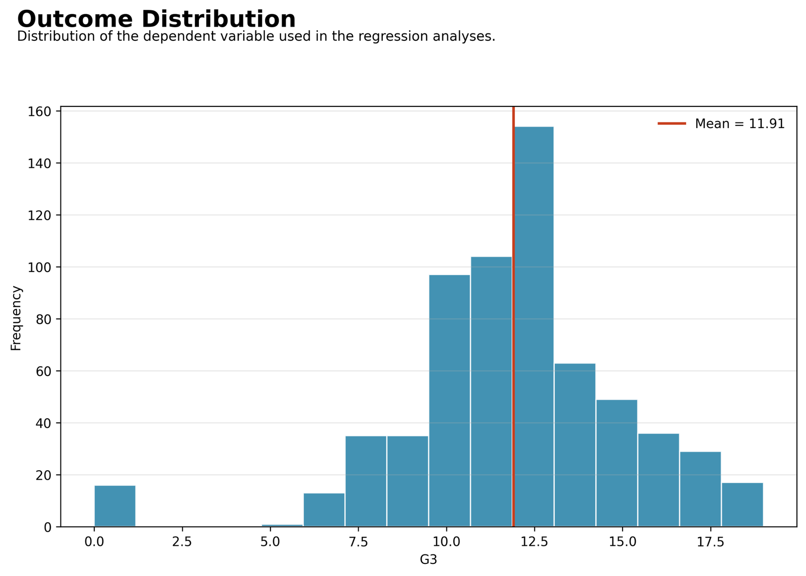
The bounded integer outcome is concentrated in the middle grades with a tail at zero, a shape that helps explain later residual non-normality.
Confirm N = 649 and the plotted column is G3.
Python chart 1: G3 outcome distribution.
Review skew, boundary concentrations, sparse cells, and tail observations before choosing or interpreting the Regression in Python model.
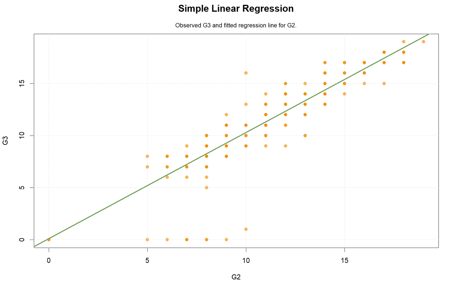
Python Chart 2: Simple scatterplot with fitted line
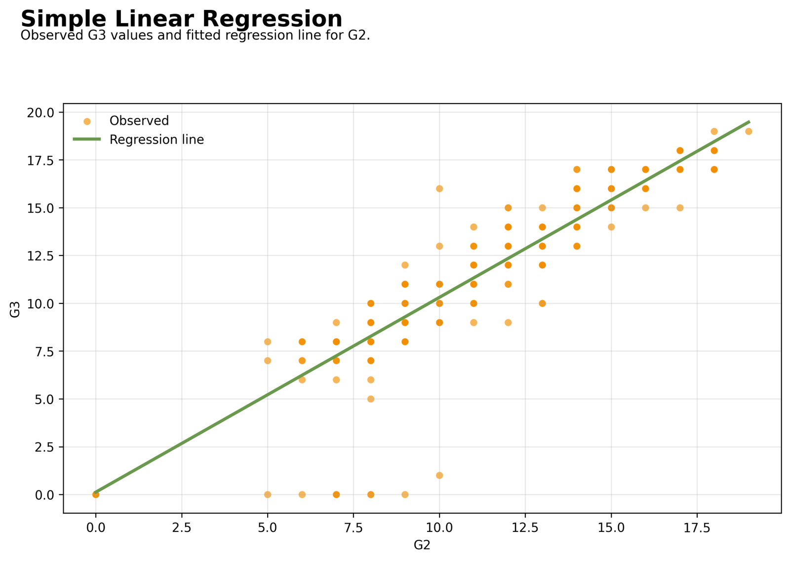
The strong G2-G3 alignment matches R-squared 0.843730, while departures from the line remain visible as individual errors.
Match the line to intercept 0.121966 and slope 1.018490.
Python chart 2: Simple scatterplot with fitted line.
Check departures from the reference line across the full fitted range and verify the corresponding Regression in Python error metrics.
Python Chart 3: Multiple-model observed versus predicted
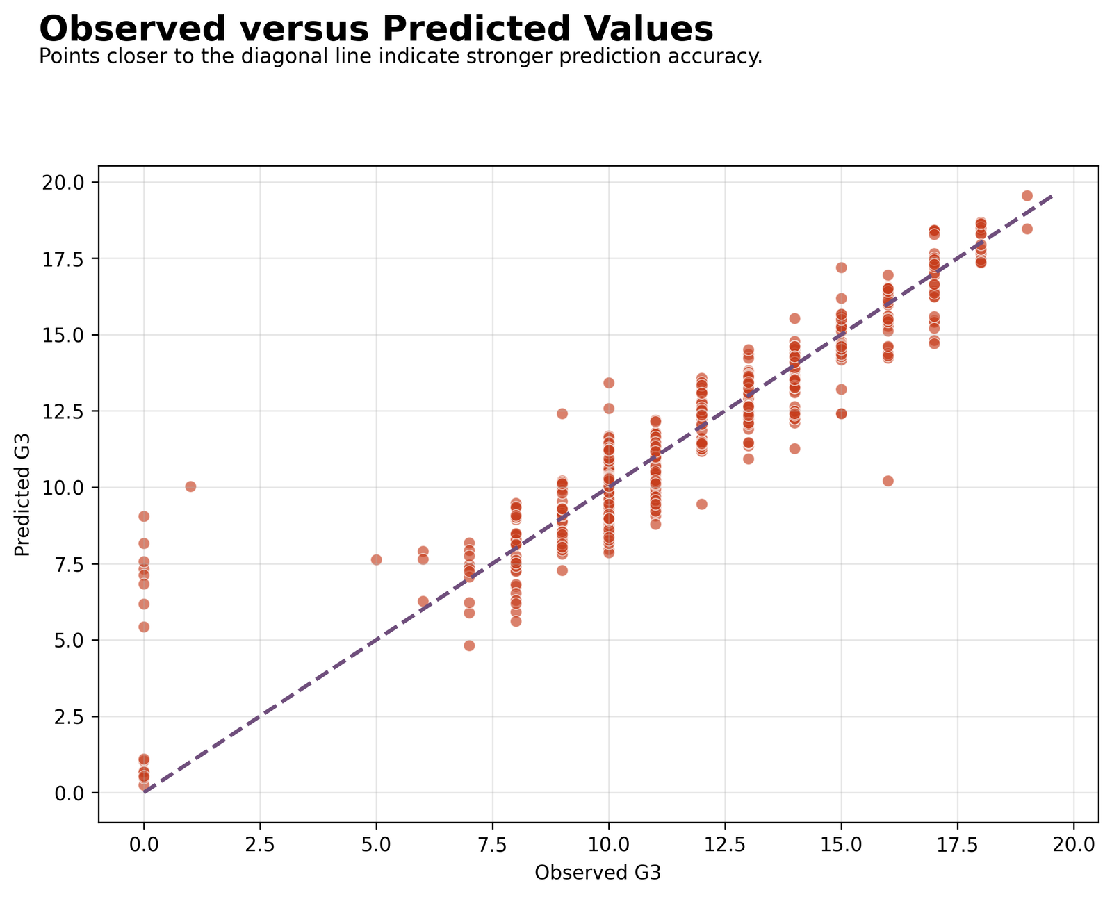
The diagonal relation reflects the 0.850777 fitted R-squared; points away from identity identify under- and over-prediction.
Use predictions from the eight-predictor fit only.
Python chart 3: Multiple-model observed versus predicted.
Check departures from the reference line across the full fitted range and verify the corresponding Regression in Python error metrics.
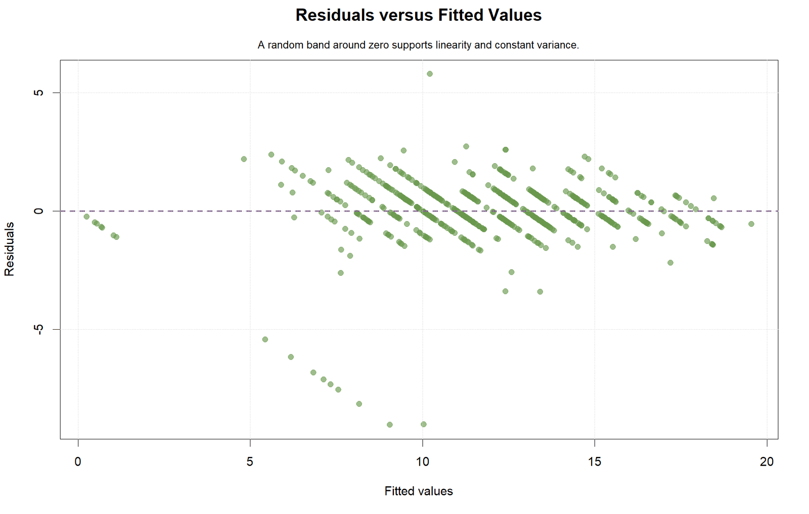
Python Chart 4: Multiple residuals versus fitted
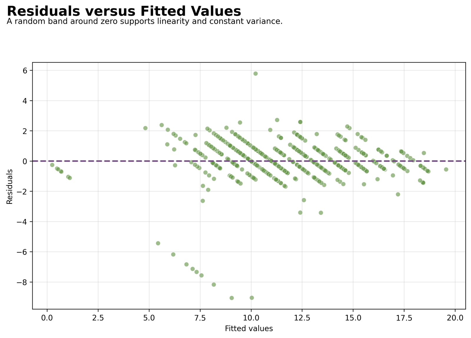
The graph assesses curvature and changing variance and should be read with the significant Breusch-Pagan result.
Residuals must equal observed minus fitted.
Python chart 4: Multiple residuals versus fitted.
For Regression in Python, inspect centering around zero, changing spread, curvature, and individual cases before accepting the residual pattern.
Python Chart 5: Multiple residual histogram
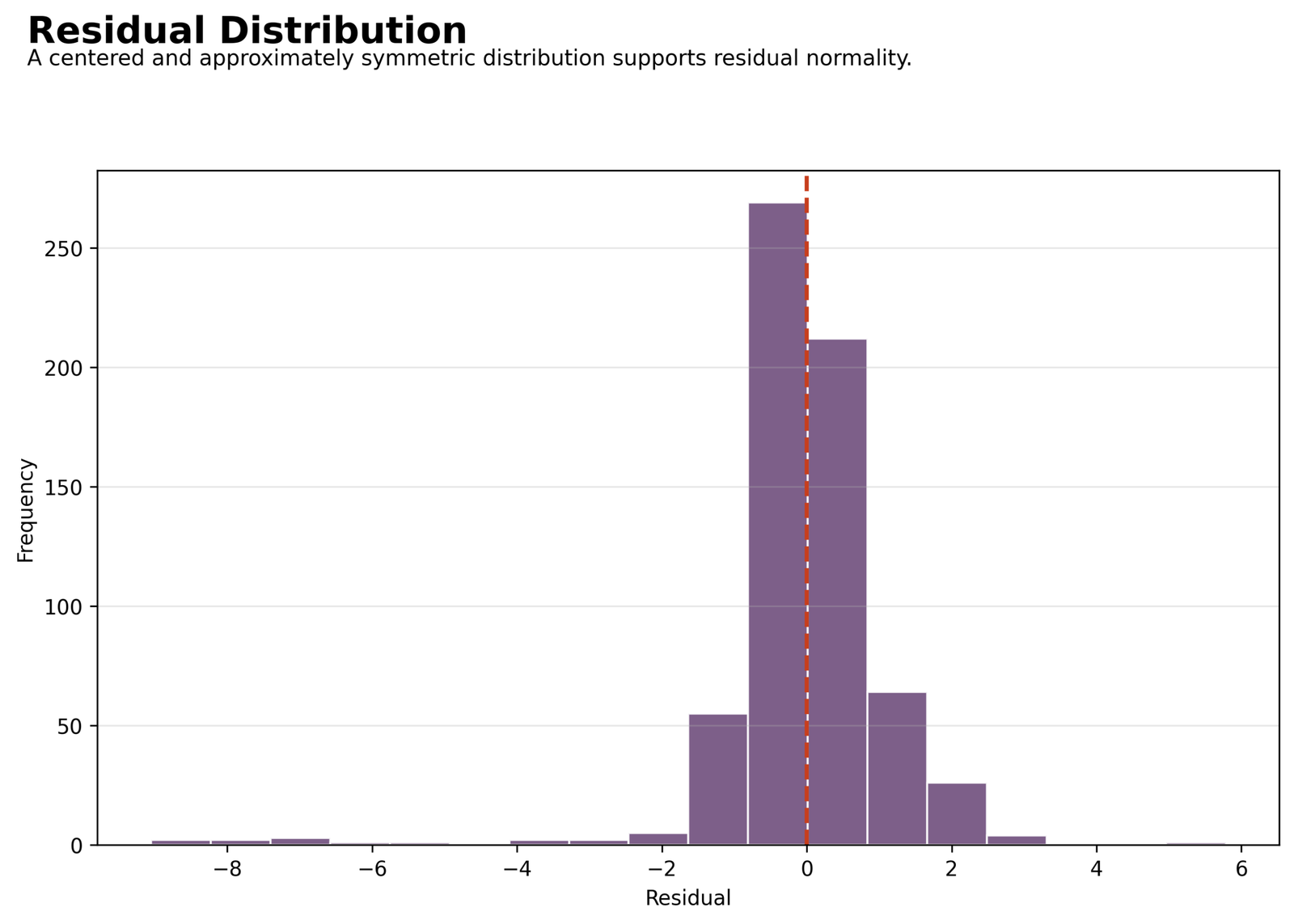
The distribution centers near zero but has a non-normal tail, consistent with formal normality tests.
Check the histogram uses multiple-model residuals.
Python chart 5: Multiple residual histogram.
For Regression in Python, inspect centering around zero, changing spread, curvature, and individual cases before accepting the residual pattern.
Python Chart 6: Multiple residual Q-Q plot
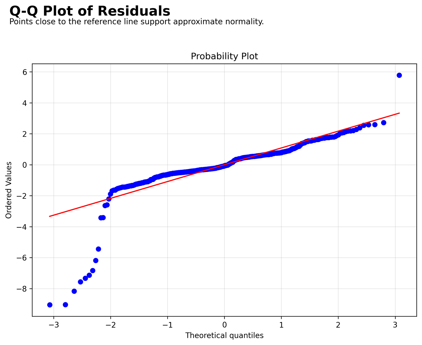
Tail departures provide visual context for Shapiro-Wilk 0.756793 and Jarque-Bera 9992.999898.
Do not interpret central alignment as full normality.
Python chart 6: Multiple residual Q-Q plot.
For Regression in Python, inspect centering around zero, changing spread, curvature, and individual cases before accepting the residual pattern.
Python Chart 7: Standardized beta ranking
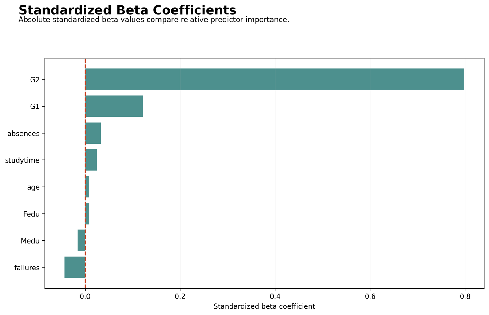
G2 at 0.797983 is dominant, followed by G1 at 0.121852; signs and magnitudes match the coefficient CSV.
Compare labels against the multiple model only.
Python chart 7: Standardized beta ranking.
Read every interval against its null reference and reconcile the plotted estimate with the exact Regression in Python coefficient table.
Python Chart 8: Simple and multiple fit comparison
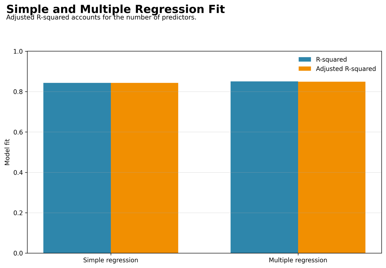
The figure shows the modest gain from adding the remaining predictors beyond G2.
Use identical observed G3 rows for both layers.
Python chart 8: Simple and multiple fit comparison.
Reconcile every displayed criterion with the exact Regression in Python results table and apply the stated selection rule consistently.
Python Chart 9: Leverage and Cook’s distance review
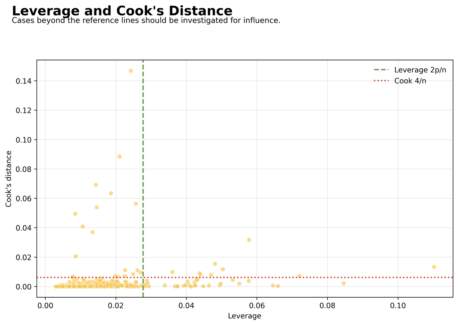
The influence panel highlights observations for investigation without prescribing automatic removal.
Trace flagged points to the case-level CSV.
Python chart 9: Leverage and Cook’s distance review.
Open the case-level Regression in Python audit and inspect every observation that crosses the stated influence or leverage threshold.
Python Chart 10: Predictor correlation heatmap
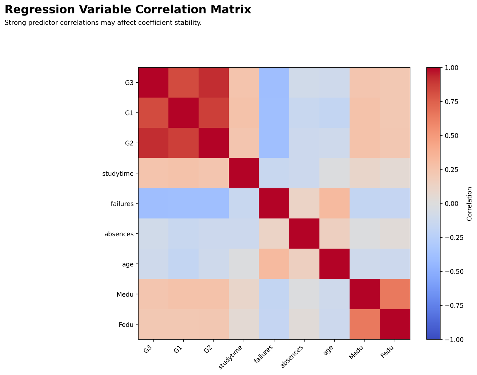
The strong G1-G2 overlap explains their VIF values near four and provides context for conditional coefficients.
Verify every heatmap label matches the modeled columns.
Python chart 10: Predictor correlation heatmap.
Cross-check this predictor correlation heatmap against the exact Regression in Python table, its companion software output, and the stated diagnostic rule.
R Charts and Explanations
The R visuals use the same worked data and are arranged as paired charts with one matching explanation beneath each graph. Values are cross-checked against the Regression in Python R tables and report.
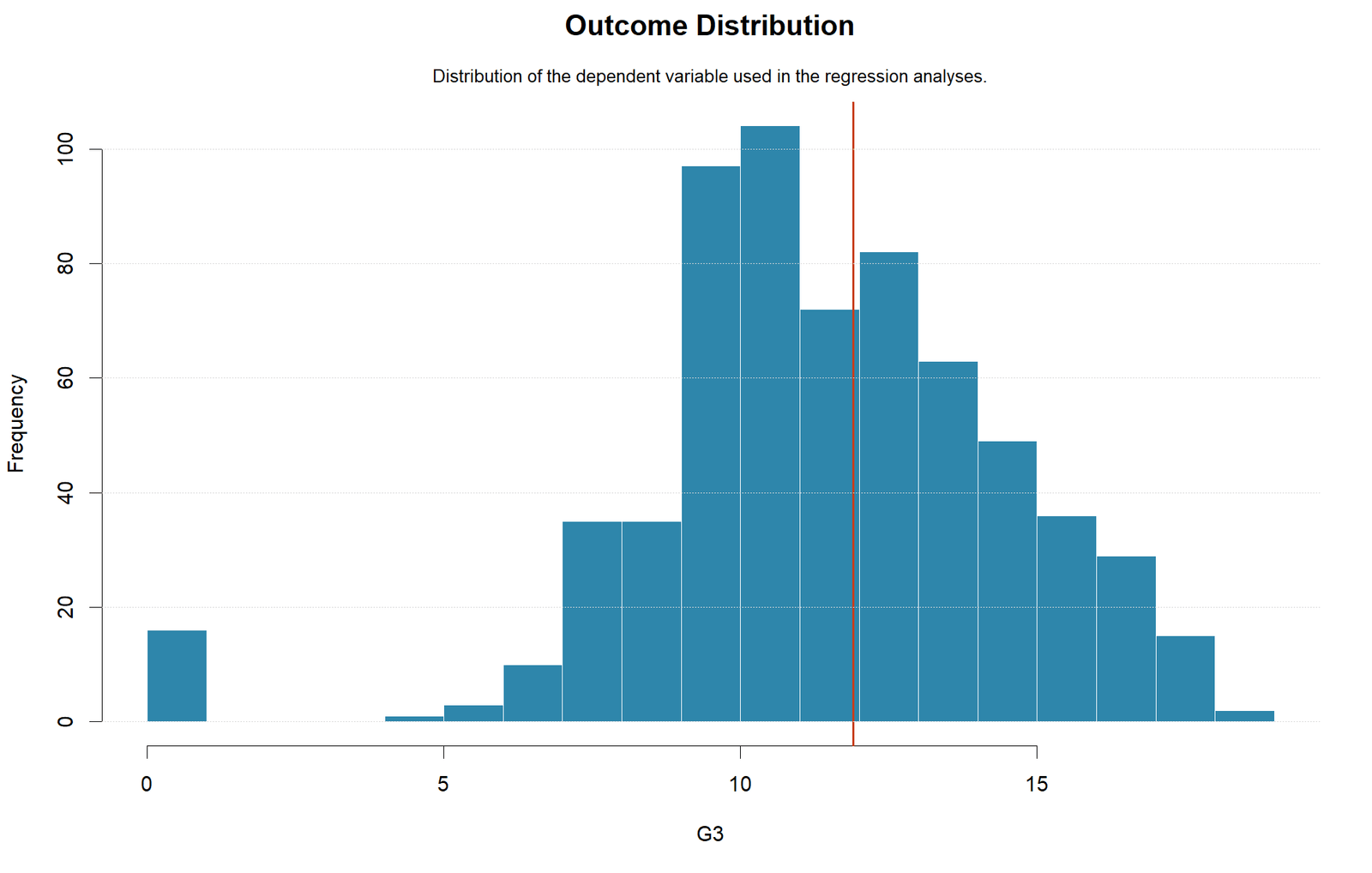
R Chart 1: G3 outcome distribution
The bounded integer outcome is concentrated in the middle grades with a tail at zero, a shape that helps explain later residual non-normality. Confirm N = 649 and the plotted column is G3. Python chart 1: G3 outcome distribution.
R Chart 2: Simple scatterplot with fitted line
The strong G2-G3 alignment matches R-squared 0.843730, while departures from the line remain visible as individual errors. Match the line to intercept 0.121966 and slope 1.018490. Python chart 2: Simple scatterplot with fitted line.
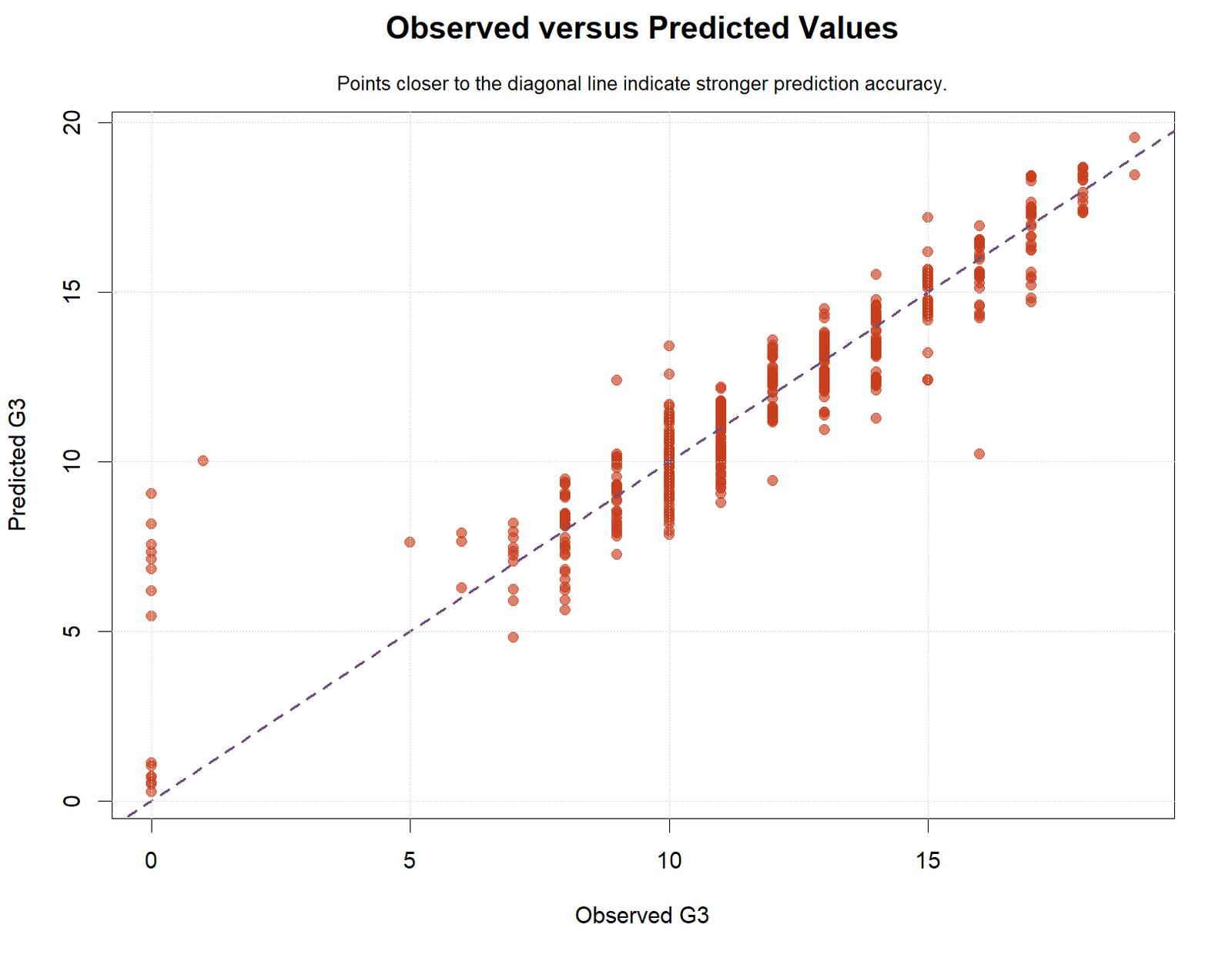
R Chart 3: Multiple-model observed versus predicted
The diagonal relation reflects the 0.850777 fitted R-squared; points away from identity identify under- and over-prediction. Use predictions from the eight-predictor fit only. Python chart 3: Multiple-model observed versus predicted.
R Chart 4: Multiple residuals versus fitted
The graph assesses curvature and changing variance and should be read with the significant Breusch-Pagan result. Residuals must equal observed minus fitted. Python chart 4: Multiple residuals versus fitted.
Regression in Python Coefficient and Parameter Interpretation
Verified Coefficient Evidence Table
Statsmodels params retain grade-point units, whereas the exported beta calculation rescales slopes using the dataframe standard deviations.
| Term | B | SE | t | p | 95% CI | Beta |
|---|---|---|---|---|---|---|
| Intercept | -0.501155 | 0.773950 | -0.6475 | 0.5175 | [-2.0209, 1.0186] | – |
| G1 | 0.143397 | 0.036672 | 3.9103 | 0.000102 | [0.0714, 0.2154] | 0.121852 |
| G2 | 0.884807 | 0.034369 | 25.7440 | 7.355e-101 | [0.8173, 0.9523] | 0.797983 |
| studytime | 0.096632 | 0.062091 | 1.5563 | 0.1201 | [-0.0253, 0.2186] | 0.024811 |
| failures | -0.235361 | 0.095234 | -2.4714 | 0.0137 | [-0.4224, -0.0484] | -0.043219 |
| absences | 0.022762 | 0.010919 | 2.0846 | 0.0375 | [0.0013, 0.0442] | 0.032697 |
| age | 0.022685 | 0.043668 | 0.5195 | 0.6036 | [-0.0631, 0.1084] | 0.008554 |
| Medu | -0.044951 | 0.057938 | -0.7759 | 0.4381 | [-0.1587, 0.0688] | -0.015786 |
| Fedu | 0.022025 | 0.059316 | 0.3713 | 0.7105 | [-0.0945, 0.1385] | 0.007499 |
Coefficient Inference from Python
Python checkpoint. how estimate, standard error, t statistic, p value and interval fit together. The output gives B = 0.884807 for G2 with a 95 percent interval from 0.817317 to 0.952298; failures is -0.235361 with interval -0.422371 to -0.048351.
Statistical reading. The sign and interval describe conditional association; the p value measures compatibility with a zero coefficient under the model assumptions.
Decision rule. Prioritize interval magnitude and subject interpretation over a binary significance column.
Verification step 6. Check that each table row belongs to the multiple model before quoting it, because the CSV also stores simple-model coefficients.
Evidence to retain for this section
The output gives B = 0.884807 for G2 with a 95 percent interval from 0.817317 to 0.952298; failures is -0.235361 with interval -0.422371 to -0.048351.
Failure mode to avoid
Predictions, Effects and Model Meaning
Predictions from Regression in Python inherit the fitted equation, coding, link or transformation, and training-data conventions documented above. Python chart 1: G3 outcome distribution.
Regression in Python Assumptions and Diagnostics
Residual Normality Tests
Python checkpoint. how formal tests qualify the histogram and Q-Q plot. For the multiple fit, Shapiro-Wilk is 0.756793 with p = 7.918e-30 and Jarque-Bera is 9992.999898 with p reported as zero.
Statistical reading. Both tests flag non-normal residual shape, consistent with bounded integer grades and extreme negative errors in the plotted tail.
Decision rule. Do not erase the result because the model is large; discuss robust inference or prediction-focused validation where appropriate.
Verification step 9. Match the test row’s model label to the multiple residual histogram and Q-Q filenames.
Evidence to retain for this section
For the multiple fit, Shapiro-Wilk is 0.756793 with p = 7.918e-30 and Jarque-Bera is 9992.999898 with p reported as zero.
Failure mode to avoid
Heteroscedasticity Evidence
Python checkpoint. whether residual spread is constant across fitted values. The multiple-model Breusch-Pagan statistic is 35.722807 with p = 1.9735e-05, and its F version is 4.659923 with p = 1.4815e-05.
Statistical reading. The tests indicate changing variance, so conventional OLS standard errors deserve caution even though point predictions remain computable.
Decision rule. Consider heteroscedasticity-robust covariance for inference and show the residual-versus-fitted plot in the report.
Verification step 10. Keep the original and robust uncertainty results separately labeled if the script is extended.
Evidence to retain for this section
The multiple-model Breusch-Pagan statistic is 35.722807 with p = 1.9735e-05, and its F version is 4.659923 with p = 1.4815e-05.
Failure mode to avoid
Residual Independence and Ordering
Python checkpoint. what Durbin-Watson contributes to the review. The saved multiple-model Durbin-Watson value is 1.861535, described as near the approximate independence reference of two.
Statistical reading. The statistic only has a meaningful ordering interpretation when row sequence represents time or another coherent order.
Decision rule. Report the value cautiously and rely on the study design to decide whether clustered or longitudinal methods are needed.
Verification step 11. Confirm the dataset was not arbitrarily sorted immediately before the diagnostic was calculated.
Evidence to retain for this section
The saved multiple-model Durbin-Watson value is 1.861535, described as near the approximate independence reference of two.
Failure mode to avoid
Regression in Python in Python, R, SPSS and Excel
Python Model Question and Scope
Python checkpoint. how the script separates a one-predictor demonstration from the adjusted model. The executed report names G3 as the outcome, G2 as the simple predictor and eight columns in the multiple formula. It records 649 original and used rows.
Statistical reading. The two fits answer different questions and are preserved as separate table rows, coefficient blocks and diagnostic series.
Decision rule. Choose the formula before inspecting p values and keep the simple comparison descriptive when the adjusted model is primary.
Verification step 1. Read the exact formula strings from the saved report and coefficient CSV rather than reconstructing them from chart labels.
Evidence to retain for this section
The executed report names G3 as the outcome, G2 as the simple predictor and eight columns in the multiple formula. It records 649 original and used rows.
Failure mode to avoid
Simple Python Fit
Python checkpoint. what the one-column model demonstrates. For G3 on G2, R-squared is 0.843730, adjusted R-squared is 0.843489, F is 3493.281566, RMSE is 1.276125 and MAE is 0.808023.
Statistical reading. The slope 1.018490 captures a strong direct relationship, while the residual diagnostics show that a strong line can still have non-normal and nonconstant errors.
Decision rule. Use the simple fit to explain slope geometry, not to claim that G2 alone is a complete data-generating account.
Verification step 4. Verify the scatter-line chart uses the simple prediction column and the coefficient row labeled Simple linear regression.
Evidence to retain for this section
For G3 on G2, R-squared is 0.843730, adjusted R-squared is 0.843489, F is 3493.281566, RMSE is 1.276125 and MAE is 0.808023.
Failure mode to avoid
Multiple Python Fit
Python checkpoint. how the adjusted estimates change the story.
Statistical reading. Adding seven predictors beyond G2 yields a smaller error and modest fit increase; G2 nevertheless remains the dominant standardized predictor.
Decision rule. Report the complete formula and distinguish in-sample error from expected error on unseen records.
Verification step 5. Recalculate RMSE from the saved prediction-residual table and compare it with the model-comparison CSV.
Evidence to retain for this section
Failure mode to avoid
Influence Diagnostics in Python
Python checkpoint. how leverage and Cook’s distance identify cases worth inspection. The predictions-residuals-influence table and ninth chart store leverage and Cook’s distance for every used row.
Statistical reading. A high value is a review flag rather than an automatic deletion command; an unusual but valid student can be substantively important.
Decision rule. Repeat the fit with documented sensitivity checks when a case appears influential.
Verification step 12. Trace any plotted extreme back to its case row and verify its source values before modifying the analysis.
Evidence to retain for this section
The predictions-residuals-influence table and ninth chart store leverage and Cook’s distance for every used row.
Failure mode to avoid
Python Reproducibility Record
Python checkpoint. which outputs make the analysis auditable. The folder contains the executed script, ten CSV tables, ten PNG charts, a PDF report and a short text report.
Statistical reading. This separation allows readers to inspect machine-readable coefficients independently from rendered figures and narrative summaries.
Decision rule. Version the script and outputs together so later edits cannot leave stale charts beside new tables.
Verification step 14. Compare file modification times and regenerate the complete output set in one run after any code change.
Evidence to retain for this section
The folder contains the executed script, ten CSV tables, ten PNG charts, a PDF report and a short text report.
Failure mode to avoid
Python Decision and Next Analysis
Python checkpoint. what the verified output supports after diagnostics are considered. The model provides strong in-sample fit and a stable dominant G2 association, but residual tests flag shape and variance problems.
Statistical reading. The evidence supports a useful conditional prediction equation with caveats; it does not establish causal effects or guarantee transport to a new school population.
Decision rule. Use a held-out set or resampling pipeline for generalization and compare robust standard errors for inference.
Verification step 16. Preserve the current verified outputs as a benchmark before making any extension.
Evidence to retain for this section
The model provides strong in-sample fit and a stable dominant G2 association, but residual tests flag shape and variance problems.
Failure mode to avoid
Software Workflows and Reproducibility
pandas
Loads and validates the model columns and stores case-level evidence.
statsmodels
Fits OLS, confidence intervals, residual tests and influence measures.
matplotlib
Renders the saved diagnostic figures with explicit labels.
scikit-learn
Can add held-out or cross-validated prediction assessment without replacing the fitted inference object.
Regression in Python Assumptions and Data-Pipeline Preconditions
Linearity concerns the conditional mean of G3 given the predictors, not whether each raw variable has a normal histogram. The residuals-versus-fitted image is the first visual check for curvature, but discrete grade bands and the lower bound at zero complicate its appearance. A systematic arc would suggest transformations, polynomial terms or interactions; a few isolated negative residuals near zero grades suggest a different issue. The script should preserve both the plot and the exact residual table so a visual pattern can be connected to records rather than judged from pixels alone.
Independence comes from how student records were collected. Durbin-Watson 1.861535 is close to the reference value two, yet it only summarizes first-order correlation in the current row order. It cannot rule out clustering within schools, classes or households, and shuffling the dataframe would change its interpretation without changing any coefficient. Before relying on classical standard errors, the analyst must decide whether the sampling design supplies genuinely independent units or whether cluster-aware covariance or a multilevel model is warranted.
Constant conditional variance is not supported by the stored multiple-model diagnostics. Breusch-Pagan is 35.7228073187 with p = 1.9734996372e-05, and its F form is 4.6599231467 with p = 1.4815229235e-05. Those values indicate that residual spread varies with the design variables under the test specification. The OLS coefficient vector can still describe the fitted conditional mean, but classical standard errors and intervals need qualification; an HC3 covariance sensitivity analysis would address uncertainty without pretending to repair mean-form errors.
Residual normality is also doubtful. The multiple Shapiro-Wilk statistic is 0.7567934286 with p = 7.9184674073e-30, while Jarque-Bera is 9992.9998983527 with probability reported as zero at machine precision. The histogram and Q Q plot show why: several zero final grades create an unusually long negative tail. Large n can stabilize many coefficient estimates, but it does not make tail behavior irrelevant for individual prediction intervals, outlier diagnostics or claims that depend on a Gaussian likelihood.
Multicollinearity is a property of the predictor design. G1 has VIF 4.1648316426 and G2 has 4.1207954322, reflecting substantial overlap between two earlier grade measures; all other reported VIF values are below 1.78. These numbers do not require automatic deletion. They explain why conditional slopes and their standard errors differ from bivariate relationships, and they motivate coefficient-stability checks when one prior grade is removed or when the model is refit on resampled data.
Influential observations require a combined reading of residual size and predictor-space leverage. Case 1 has leverage 0.1102142948, much larger than an average diagonal value for a nine-parameter design, but Cook distance 0.0133658751 must be interpreted relative to the complete distribution and the coefficient changes it induces. A high value triggers source verification and a fit-without-case sensitivity analysis. It does not license silent deletion, especially when the row may represent a valid combination such as G1 equal to zero followed by later grades.
Data-pipeline assumptions precede model assumptions. Required columns must be numeric, categories must be encoded consistently, missing rows must be handled once, and the response cannot leak into predictor construction. The report states 649 original rows and 649 used rows, so any rerun returning a different count has already diverged from the verified analysis. Assertions on column presence, dtype, finite values, row identifiers and final N should fail loudly before OLS is allowed to fit.
Python Software Procedure, Saved Output and Clean Rerun
A clean run begins by resolving the same-topic dataset path and reading it with pandas. The script should print the resolved path, row count, column names and a concise dtype summary before selecting variables. Assertions then require G3 and all predictors, reject duplicate row identifiers, and verify finite numeric values. These checks make a wrong-file execution obvious before it can generate credible-looking regression tables.
The simple and multiple matrices should be built in separate named variables. After add_constant, each model is passed to sm.OLS and fit once, producing distinct result objects such as simple_result and multiple_result. Reusing a generic variable named model for both stages encourages accidental exports from the wrong fit. Explicit names also make figure titles and filenames easier to generate without cross-topic substitution.
Structured extraction follows fitting. A coefficient dataframe can combine params, bse, tvalues, pvalues and conf_int by index; a model-comparison row can read nobs, rsquared, rsquared_adj, fvalue, f_pvalue, AIC, BIC and residual metrics. VIF is calculated from the multiple exogenous matrix with the intercept excluded from substantive interpretation. Every export should include a model label so a later join cannot mix simple and multiple rows.
Diagnostics require additional result APIs and functions. Predictions and intervals come from get_prediction, influence values from get_influence or OLSInfluence, Durbin-Watson from the residual array, and Breusch-Pagan from residuals plus the multiple exogenous matrix. Normality functions should receive exactly the residual vector named in the table. Recording function inputs and model labels prevents a simple-model test from appearing under a multiple-model caption.
Chart generation should consume saved tables or the same in-memory arrays used to create them. Axis labels need variable names and units, legends must identify simple versus multiple fits, and annotations should be derived from result values rather than typed. Saving a figure with a stable topic-specific filename is only half the job; the meta mapping must also identify Python so duplicate basenames from R cannot be selected accidentally.
The report assembly stage reads the generated evidence and states software-specific limitations. It should not scrape its own PNG labels for numbers, and it should exclude broad-match, SERP and transcript files even when they share topic words. A manifest listing each output filename, originating object and checksum would make the connection between code, CSV, image and PDF independently reviewable.
Verification ends with deletion or isolation of prior generated outputs, a restart from a clean interpreter, and comparison against anchor values. The rerun should recover 649 used rows, multiple R-squared 0.8507771982, G2 B 0.8848073756, Breusch-Pagan 35.7228073187 and the documented case 1 prediction. If an anchor moves, the analyst investigates data, versions and code before publication rather than editing the output to match.
Code: Expand Only the Software You Need
Standardized Effects in Code
Python checkpoint. how the script compares predictors measured on different scales. G2 has standardized beta 0.797983, G1 has 0.121852 and the remaining absolute beta values are below 0.044 in the saved model.
Statistical reading. The standardized display is a transformation of the fitted slopes and observed standard deviations, not a separate regression.
Decision rule. Use standardized betas to discuss relative modeled strength while retaining B for practical unit changes.
Verification step 7. Compare the chart values with the absolute_standardized_beta column rather than sorting on raw B.
Evidence to retain for this section
G2 has standardized beta 0.797983, G1 has 0.121852 and the remaining absolute beta values are below 0.044 in the saved model.
Failure mode to avoid
Code and Formula Blocks
Statsmodels multiple OLS
import pandas as pd
import statsmodels.api as sm

df = pd.read_csv("dataset.csv")
cols = ["G1","G2","studytime","failures","absences","age","Medu","Fedu"]
X = sm.add_constant(df[cols], has_constant="add")
fit = sm.OLS(df["G3"], X, missing="drop").fit()
pred = fit.predict(X)
resid = df.loc[pred.index, "G3"] - pred
print(fit.summary())
This code panel mirrors the pandas and statsmodels operations used by the topic script.
Robust uncertainty check
robust = fit.get_robustcov_results(cov_type="HC3")
print(robust.summary())
This block expresses the method used by the topic.
Verified Python Core Implementation
def prepare_data(
data: pd.DataFrame,
) -> tuple[pd.DataFrame, str, str, list[str]]:
outcome = choose_outcome(data)
simple_predictor = choose_simple_predictor(data, outcome)
multiple_predictors = choose_multiple_predictors(
data,
outcome,
simple_predictor,
)
keep_columns = [outcome] + list(
dict.fromkeys([simple_predictor] + multiple_predictors)
)
analysis_data = data[keep_columns].copy()
for column in analysis_data.columns:
analysis_data[column] = pd.to_numeric(
analysis_data[column],
errors="coerce",
)
analysis_data = (
analysis_data
.replace([np.inf, -np.inf], np.nan)
.dropna()
.reset_index(drop=True)
)
if len(analysis_data) <= len(multiple_predictors) + 10:
raise ValueError(
"Not enough complete observations for the requested regression models."
)
return (
analysis_data,
outcome,
simple_predictor,
multiple_predictors,
)
def fit_ols(
data: pd.DataFrame,
outcome: str,
predictors: list[str],
):
y = data[outcome].astype(float)
x = sm.add_constant(
data[predictors].astype(float),
has_constant="add",
)
return sm.OLS(y, x).fit()
def make_model_summary(
result,
model_name: str,
outcome: str,
predictors: list[str],
) -> pd.DataFrame:
residuals = np.asarray(result.resid, dtype=float)
return pd.DataFrame(
[
{
"model": model_name,
"outcome": outcome,
"predictors": ", ".join(predictors),
"observations": int(result.nobs),
"number_of_predictors": len(predictors),
"r_squared": float(result.rsquared),
"adjusted_r_squared": float(result.rsquared_adj),
"f_statistic": float(result.fvalue),
"f_p_value": float(result.f_pvalue),
"aic": float(result.aic),
"bic": float(result.bic),
"rmse": float(np.sqrt(np.mean(residuals ** 2))),
"mae": float(np.mean(np.abs(residuals))),
"residual_standard_error": float(
np.sqrt(np.sum(residuals ** 2) / result.df_resid)
),
"durbin_watson": float(durbin_watson(residuals)),
"decision_alpha_0_05": (
"Model is statistically significant"
if result.f_pvalue < ALPHA
else "Model is not statistically significant"
),
}
]
)
def make_coefficient_table(
result,
model_name: str,
outcome_standard_deviation: float,
predictor_standard_deviations: dict[str, float],
) -> pd.DataFrame:
confidence_intervals = result.conf_int(alpha=ALPHA)
rows: list[dict] = []
for term in result.params.index:
coefficient = float(result.params[term])
standard_error = float(result.bse[term])
t_value = float(result.tvalues[term])
p_value = float(result.pvalues[term])
lower = float(confidence_intervals.loc[term, 0])
upper = float(confidence_intervals.loc[term, 1])
display_term = "Intercept" if term == "const" else term
if term == "const":
standardized_beta = np.nan
else:
standardized_beta = (
coefficient
* predictor_standard_deviations[term]
/ outcome_standard_deviation
)
rows.append(
{
"model": model_name,
"term": display_term,
"coefficient_b": coefficient,
"standard_error": standard_error,
"t_value": t_value,
"p_value": p_value,
"ci95_lower": lower,
"ci95_upper": upper,
"standardized_beta": standardized_beta,
"absolute_standardized_beta": (
abs(standardized_beta)
if np.isfinite(standardized_beta)
else np.nan
),
"decision_alpha_0_05": (
"Statistically significant"
if p_value < ALPHA
else "Not statistically significant"
),
}
)
return pd.DataFrame(rows)
def make_anova_table(result, model_name: str) -> pd.DataFrame:
observed = np.asarray(result.model.endog, dtype=float)
fitted = np.asarray(result.fittedvalues, dtype=float)
residuals = np.asarray(result.resid, dtype=float)
total_sum_squares = float(
np.sum((observed - np.mean(observed)) ** 2)
)
regression_sum_squares = float(
np.sum((fitted - np.mean(observed)) ** 2)
)
residual_sum_squares = float(
np.sum(residuals ** 2)
)
regression_df = int(result.df_model)
residual_df = int(result.df_resid)
total_df = regression_df + residual_df
regression_mean_square = (
regression_sum_squares / regression_df
if regression_df > 0
else np.nan
)
residual_mean_square = (
residual_sum_squares / residual_df
if residual_df > 0
else np.nan
)
return pd.DataFrame(
[
{
"model": model_name,
"source": "Regression",
"sum_of_squares": regression_sum_squares,
"df": regression_df,
"mean_square": regression_mean_square,
"f_value": float(result.fvalue),
"p_value": float(result.f_pvalue),
},
{
"model": model_name,
"source": "Residual",
"sum_of_squares": residual_sum_squares,
"df": residual_df,
"mean_square": residual_mean_square,
"f_value": np.nan,
"p_value": np.nan,
},
{
"model": model_name,
"source": "Total",
"sum_of_squares": total_sum_squares,
"df": total_df,
"mean_square": np.nan,
"f_value": np.nan,
"p_value": np.nan,
},
]
)
def make_vif_table(
data: pd.DataFrame,
predictors: list[str],
) -> pd.DataFrame:
design = sm.add_constant(
data[predictors].astype(float),
has_constant="add",
)
rows: list[dict] = []
for index, term in enumerate(design.columns):
if term == "const":
continue
vif = float(
variance_inflation_factor(
design.to_numpy(dtype=float),
index,
)
)
rows.append(
{
"predictor": term,
"vif": vif,
"tolerance": 1 / vif if vif != 0 else np.nan,
"diagnostic": (
"Potential multicollinearity"
if vif >= 5
else "Acceptable"
),
}
)
return pd.DataFrame(rows)
def make_diagnostic_tests(
result,
model_name: str,
) -> pd.DataFrame:
residuals = np.asarray(result.resid, dtype=float)
exogenous = np.asarray(result.model.exog, dtype=float)
if len(residuals) >= 3:
shapiro_statistic, shapiro_p_value = stats.shapiro(
residuals[:5000]
)
else:
shapiro_statistic, shapiro_p_value = np.nan, np.nan
jarque_bera = stats.jarque_bera(residuals)
try:
bp_statistic, bp_p_value, bp_f_statistic, bp_f_p_value = (
het_breuschpagan(
residuals,
exogenous,
)
)
except Exception:
bp_statistic = np.nan
bp_p_value = np.nan
bp_f_statistic = np.nan
bp_f_p_value = np.nan
return pd.DataFrame(
[
{
"model": model_name,
"diagnostic": "Shapiro-Wilk residual normality",
"statistic": shapiro_statistic,
"p_value": shapiro_p_value,
"interpretation": (
"Potential non-normality"
if shapiro_p_value < ALPHA
else "No strong evidence against normality"
),
},
{
"model": model_name,
"diagnostic": "Jarque-Bera residual normality",
"statistic": jarque_bera.statistic,
"p_value": jarque_bera.pvalue,
"interpretation": (
"Potential non-normality"
if jarque_bera.pvalue < ALPHA
else "No strong evidence against normality"
),
},
{
"model": model_name,
"diagnostic": "Breusch-Pagan heteroscedasticity",
"statistic": bp_statistic,
"p_value": bp_p_value,
"interpretation": (
"Potential heteroscedasticity"
if bp_p_value < ALPHA
else "No strong evidence of heteroscedasticity"
),
},
{
"model": model_name,
"diagnostic": "Breusch-Pagan F test",
"statistic": bp_f_statistic,
"p_value": bp_f_p_value,
"interpretation": (
"Potential heteroscedasticity"
if bp_f_p_value < ALPHA
else "No strong evidence of heteroscedasticity"
),
},
{
"model": model_name,
"diagnostic": "Durbin-Watson residual independence",
"statistic": float(durbin_watson(residuals)),
"p_value": np.nan,
"interpretation": (
"Values near 2 indicate approximate independence"
),
},
]
)
def make_prediction_table(
data: pd.DataFrame,
outcome: str,
simple_predictor: str,
multiple_predictors: list[str],
simple_result,
multiple_result,
) -> pd.DataFrame:
multiple_influence = multiple_result.get_influence()
prediction_frame = multiple_result.get_prediction().summary_frame(
alpha=ALPHA
)
output = data[
[outcome] + list(
dict.fromkeys([simple_predictor] + multiple_predictors)
)
].copy()
output.insert(
0,
"case_number",
np.arange(1, len(output) + 1),
)
output["simple_predicted_value"] = (
simple_result.fittedvalues.to_numpy()
)
output["simple_residual"] = (
simple_result.resid.to_numpy()
)
output["multiple_predicted_value"] = (
multiple_result.fittedvalues.to_numpy()
)
output["multiple_residual"] = (
multiple_result.resid.to_numpy()
)
output["multiple_standardized_residual"] = (
multiple_influence.resid_studentized_internal
)
output["multiple_external_studentized_residual"] = (
multiple_influence.resid_studentized_external
)
output["multiple_leverage"] = (
multiple_influence.hat_matrix_diag
)
output["multiple_cooks_distance"] = (
multiple_influence.cooks_distance[0]
)
output["multiple_dffits"] = (
multiple_influence.dffits[0]
)
output["mean_ci_lower_95"] = prediction_frame["mean_ci_lower"].to_numpy()
output["mean_ci_upper_95"] = prediction_frame["mean_ci_upper"].to_numpy()
output["prediction_interval_lower_95"] = (
prediction_frame["obs_ci_lower"].to_numpy()
)
output["prediction_interval_upper_95"] = (
prediction_frame["obs_ci_upper"].to_numpy()
)
return output
def add_title_and_subtitle(
figure,
title: str,
subtitle: str,
) -> None:
figure.suptitle(
title,
x=0.06,
y=0.975,
ha="left",
fontsize=18,
fontweight="bold",
)
figure.text(
0.06,
0.925,
subtitle,
ha="left",
fontsize=10.5,
)
figure.subplots_adjust(
top=0.82,
left=0.11,
right=0.95,
bottom=0.15,
)
def save_figure(
figure,
filename: str,
) -> Path:
path = PNG_DIR / filename
figure.savefig(
path,
dpi=300,
bbox_inches="tight",
)
plt.close(figure)
return path
def create_charts(
data: pd.DataFrame,
outcome: str,
simple_predictor: str,
multiple_predictors: list[str],
simple_result,
multiple_result,
simple_summary: pd.DataFrame,
multiple_summary: pd.DataFrame,
multiple_coefficients: pd.DataFrame,
predictions: pd.DataFrame,
) -> list[Path]:
charts: list[Path] = []
figure, axis = plt.subplots(figsize=(9.5, 6.8))
axis.hist(
data[outcome],
bins=16,
edgecolor="white",
alpha=0.9,
color=CHART_COLORS[0],
)
axis.axvline(
data[outcome].mean(),
linewidth=2,
color=CHART_COLORS[2],
label=f"Mean = {data[outcome].mean():.2f}",
)
axis.set_xlabel(outcome)
axis.set_ylabel("Frequency")
axis.legend(frameon=False)
axis.grid(axis="y", alpha=0.3)
add_title_and_subtitle(
figure,
"Outcome Distribution",
"Distribution of the dependent variable used in the regression analyses.",
)
charts.append(
save_figure(
figure,
"01_regression_in_python_outcome_distribution.png",
)
)
figure, axis = plt.subplots(figsize=(9.5, 6.8))
axis.scatter(
data[simple_predictor],
data[outcome],
alpha=0.65,
color=CHART_COLORS[1],
edgecolor="white",
linewidth=0.5,
label="Observed",
)
order = np.argsort(data[simple_predictor].to_numpy())
axis.plot(
data[simple_predictor].to_numpy()[order],
simple_result.fittedvalues.to_numpy()[order],
linewidth=2.5,
color=CHART_COLORS[3],
label="Regression line",
)
axis.set_xlabel(simple_predictor)
axis.set_ylabel(outcome)
axis.legend(frameon=False)
axis.grid(alpha=0.3)
add_title_and_subtitle(
figure,
"Simple Linear Regression",
f"Observed {outcome} values and fitted regression line for {simple_predictor}.",
)
charts.append(
save_figure(
figure,
"02_simple_regression_scatter_with_line.png",
)
)
figure, axis = plt.subplots(figsize=(8.5, 7))
axis.scatter(
data[outcome],
multiple_result.fittedvalues,
alpha=0.65,
color=CHART_COLORS[2],
edgecolor="white",
linewidth=0.5,
)
minimum = min(
data[outcome].min(),
multiple_result.fittedvalues.min(),
)
maximum = max(
data[outcome].max(),
multiple_result.fittedvalues.max(),
)
axis.plot(
[minimum, maximum],
[minimum, maximum],
linestyle="--",
linewidth=2,
color=CHART_COLORS[4],
)
axis.set_xlabel(f"Observed {outcome}")
axis.set_ylabel(f"Predicted {outcome}")
axis.grid(alpha=0.3)
add_title_and_subtitle(
figure,
"Observed versus Predicted Values",
"Points closer to the diagonal line indicate stronger prediction accuracy.",
)
charts.append(
save_figure(
figure,
"03_multiple_regression_observed_vs_predicted.png",
)
)
figure, axis = plt.subplots(figsize=(9.5, 6.8))
axis.scatter(
multiple_result.fittedvalues,
multiple_result.resid,
alpha=0.65,
color=CHART_COLORS[3],
edgecolor="white",
linewidth=0.5,
)
axis.axhline(
0,
linestyle="--",
linewidth=2,
color=CHART_COLORS[4],
)
axis.set_xlabel("Fitted values")
axis.set_ylabel("Residuals")
axis.grid(alpha=0.3)
add_title_and_subtitle(
figure,
"Residuals versus Fitted Values",
"A random band around zero supports linearity and constant variance.",
)
charts.append(
save_figure(
figure,
"04_multiple_regression_residuals_vs_fitted.png",
)
)
figure, axis = plt.subplots(figsize=(9.5, 6.8))
axis.hist(
multiple_result.resid,
bins=18,
edgecolor="white",
color=CHART_COLORS[4],
alpha=0.9,
)
axis.axvline(
0,
linestyle="--",
linewidth=2,
color=CHART_COLORS[2],
)
axis.set_xlabel("Residual")
axis.set_ylabel("Frequency")
axis.grid(axis="y", alpha=0.3)
add_title_and_subtitle(
figure,
"Residual Distribution",
"A centered and approximately symmetric distribution supports residual normality.",
)
charts.append(
save_figure(
figure,
"05_multiple_regression_residual_histogram.png",
)
)
figure = plt.figure(figsize=(8.5, 7))
axis = figure.add_subplot(111)
stats.probplot(
multiple_result.resid,
dist="norm",
plot=axis,
)
axis.grid(alpha=0.3)
add_title_and_subtitle(
figure,
"Q-Q Plot of Residuals",
"Points close to the reference line support approximate normality.",
)
charts.append(
save_figure(
figure,
"06_multiple_regression_residual_qq_plot.png",
)
)
coefficient_plot = (
multiple_coefficients[
multiple_coefficients["term"] != "Intercept"
]
.copy()
.sort_values("standardized_beta")
)
figure, axis = plt.subplots(
figsize=(
10.5,
max(5.5, 0.55 * len(coefficient_plot) + 2.5),
)
)
positions = np.arange(len(coefficient_plot))
axis.barh(
positions,
coefficient_plot["standardized_beta"],
color=CHART_COLORS[5],
)
axis.set_yticks(
positions,
coefficient_plot["term"],
)
axis.axvline(
0,
linestyle="--",
linewidth=1.5,
color=CHART_COLORS[2],
)
axis.set_xlabel("Standardized beta coefficient")
axis.grid(axis="x", alpha=0.3)
add_title_and_subtitle(
figure,
"Standardized Beta Coefficients",
"Absolute standardized beta values compare relative predictor importance.",
)
charts.append(
save_figure(
figure,
"07_multiple_regression_standardized_betas.png",
)
)
figure, axis = plt.subplots(figsize=(9.5, 6.8))
model_labels = ["Simple regression", "Multiple regression"]
r_squared_values = [
simple_summary.loc[0, "r_squared"],
multiple_summary.loc[0, "r_squared"],
]
adjusted_values = [
simple_summary.loc[0, "adjusted_r_squared"],
multiple_summary.loc[0, "adjusted_r_squared"],
]
x_positions = np.arange(2)
width = 0.36
axis.bar(
x_positions - width / 2,
r_squared_values,
width,
label="R-squared",
color=CHART_COLORS[0],
)
axis.bar(
x_positions + width / 2,
adjusted_values,
width,
label="Adjusted R-squared",
color=CHART_COLORS[1],
)
axis.set_xticks(
x_positions,
model_labels,
)
axis.set_ylim(
0,Report assembly and reproducible export
        min(1.05, max(r_squared_values) + 0.15),
    )
    axis.set_ylabel("Model fit")
    axis.legend(frameon=False)
    axis.grid(axis="y", alpha=0.3)
    add_title_and_subtitle(
        figure,
        "Simple and Multiple Regression Fit",
        "Adjusted R-squared accounts for the number of predictors.",
    )
    charts.append(
        save_figure(
            figure,
            "08_simple_vs_multiple_regression_fit.png",
        )
    )

    figure, axis = plt.subplots(figsize=(9.5, 6.8))
    axis.scatter(
        predictions["multiple_leverage"],
        predictions["multiple_cooks_distance"],
        alpha=0.65,
        color=CHART_COLORS[6],
        edgecolor="white",
        linewidth=0.5,
    )
    leverage_threshold = (
        2 * (len(multiple_predictors) + 1) / len(predictions)
    )
    cook_threshold = 4 / len(predictions)
    axis.axvline(
        leverage_threshold,
        linestyle="--",
        linewidth=1.8,
        label="Leverage 2p/n",
        color=CHART_COLORS[3],
    )
    axis.axhline(
        cook_threshold,
        linestyle=":",
        linewidth=1.8,
        label="Cook 4/n",
        color=CHART_COLORS[2],
    )
    axis.set_xlabel("Leverage")
    axis.set_ylabel("Cook's distance")
    axis.legend(frameon=False)
    axis.grid(alpha=0.3)
    add_title_and_subtitle(
        figure,
        "Leverage and Cook's Distance",
        "Cases beyond the reference lines should be investigated for influence.",
    )
    charts.append(
        save_figure(
            figure,
            "09_multiple_regression_influence_diagnostics.png",
        )
    )

    figure, axis = plt.subplots(figsize=(11, 9))
    correlation_matrix = data[
        [outcome] + multiple_predictors
    ].corr()

    image = axis.imshow(
        correlation_matrix,
        vmin=-1,
        vmax=1,
        cmap="coolwarm",
    )
    axis.set_xticks(
        np.arange(len(correlation_matrix.columns)),
        correlation_matrix.columns,
        rotation=45,
        ha="right",
    )
    axis.set_yticks(
        np.arange(len(correlation_matrix.index)),
        correlation_matrix.index,
    )
    figure.colorbar(
        image,
        ax=axis,
        fraction=0.046,
        pad=0.04,
        label="Correlation",
    )
    add_title_and_subtitle(
        figure,
        "Regression Variable Correlation Matrix",
        "Strong predictor correlations may affect coefficient stability.",
    )
    charts.append(
        save_figure(
            figure,
            "10_regression_variable_correlation_heatmap.png",
        )
    )

    return charts


def create_pdf_report(
    report_lines: list[str],
    tables: dict[str, pd.DataFrame],
    chart_paths: list[Path],
) -> Path:
    pdf_path = PDF_DIR / "Regression-in-Python-Report.pdf"

    with PdfPages(pdf_path) as pdf:
        figure = plt.figure(figsize=(11, 8.5))
        figure.text(
            0.06,
            0.94,
            TEST_NAME,
            fontsize=22,
            fontweight="bold",
        )

        y_position = 0.88
        for line in report_lines[:28]:
            figure.text(
                0.06,
                y_position,
                line,
                fontsize=10,
            )
            y_position -= 0.034

        pdf.savefig(
            figure,
            bbox_inches="tight",
        )
        plt.close(figure)

        for title, table_data in tables.items():
            figure, axis = plt.subplots(figsize=(11, 8.5))
            axis.axis("off")

            display = table_data.copy().head(14)

            for column in display.columns:
                if pd.api.types.is_numeric_dtype(display[column]):
                    display[column] = display[column].map(
                        lambda value: (
                            ""
                            if pd.isna(value)
                            else f"{value:.5f}"
                        )
                    )

            axis.set_title(
                title,
                fontsize=16,
                fontweight="bold",
                loc="left",
                pad=20,
            )

            table = axis.table(
                cellText=display.values,
                colLabels=display.columns,
                cellLoc="left",
                colLoc="left",
                loc="center",
            )
            table.auto_set_font_size(False)
            table.set_fontsize(6.8)
            table.scale(1, 1.2)

            pdf.savefig(
                figure,
                bbox_inches="tight",
            )
            plt.close(figure)

        for chart_path in chart_paths:
            image = plt.imread(chart_path)

            figure, axis = plt.subplots(figsize=(11, 8.5))
            axis.imshow(image)
            axis.axis("off")
            axis.set_title(
                chart_path.name,
                fontsize=13,
                fontweight="bold",
                loc="left",
            )

            pdf.savefig(
                figure,
                bbox_inches="tight",
            )
            plt.close(figure)

    return pdf_path


def main() -> None:
Advanced Regression in Python Topics
Pandas Import and Row Integrity
Python checkpoint. how data enter the pipeline without silent coercion. The saved dataset overview, variable summary and analysis-data tables document the rows and model columns used by the script.
Statistical reading. A reproducible fit depends on numeric conversion, missing-value handling and column selection occurring before the design matrix is handed to statsmodels.
Decision rule. Fail loudly when a required column is absent or contains unexpected text instead of allowing a reduced model to run.
Verification step 2. Compare the 649-row count across the overview, coefficient model metadata and predictions table.
Evidence to retain for this section
The saved dataset overview, variable summary and analysis-data tables document the rows and model columns used by the script.
Failure mode to avoid
Statsmodels OLS Design Matrix
Python checkpoint. why the intercept must be added deliberately. The coefficient output contains an intercept for both simple and multiple equations, with -0.501155 in the latter. The model includes eight slopes.
Statistical reading. An omitted constant changes residual centering, R-squared interpretation and every coefficient; adding it twice can also corrupt the intended design.
Decision rule. Construct X in an explicit column order and call add_constant once before fitting.
Verification step 3. Print exogenous names from the fitted object and reconcile them with the saved coefficient table.
Evidence to retain for this section
The coefficient output contains an intercept for both simple and multiple equations, with -0.501155 in the latter. The model includes eight slopes.
Failure mode to avoid
Variance Inflation Factors
Python checkpoint. whether the Python design shows damaging predictor redundancy. The largest VIF values are 4.164832 for G1 and 4.120795 for G2; all named predictor rows are labeled acceptable in the saved table.
Statistical reading. These values reveal substantial overlap between the two grade predictors but remain below the workflow’s closer-review threshold of five.
Decision rule. Describe the overlap and inspect stability rather than claiming that an acceptable label proves coefficients are immune to collinearity.
Verification step 8. Recompute each VIF on the same eight-column matrix and exclude the intercept from substantive interpretation.
Evidence to retain for this section
The largest VIF values are 4.164832 for G1 and 4.120795 for G2; all named predictor rows are labeled acceptable in the saved table.
Failure mode to avoid
Model Comparison without Overclaiming
Python checkpoint. how AIC, BIC and fit metrics frame the two equations. The simple model has AIC 2162.270813 and BIC 2171.221679; the multiple model has AIC 2146.324659 and BIC 2186.603553.
Statistical reading. AIC favors the multiple fit while BIC penalizes its additional parameters more strongly, demonstrating why one ranking criterion should be specified in advance.
Decision rule. Use out-of-sample validation for predictive claims instead of choosing a model solely from in-sample criteria.
Verification step 13. Keep the same rows and outcome when comparing criteria, as the saved pipeline does.
Evidence to retain for this section
The simple model has AIC 2162.270813 and BIC 2171.221679; the multiple model has AIC 2146.324659 and BIC 2186.603553.
Failure mode to avoid
Verified Chart Stories and Same-Topic Evidence
Every figure below comes from the dedicated Regression in Python folder.
Discussion of What the Python Findings Mean
The most important substantive pattern is continuity between assessment periods. G2 alone captures roughly 84 percent of fitted G3 variation, and G1 adds a smaller conditional contribution once G2 is present. This is plausible because the variables measure related academic performance at successive times. It also means that high fit partly reflects temporal proximity and overlapping measurement, not necessarily broad explanatory coverage of motivation, teaching quality or home conditions.
The multiple equation improves fitted RMSE by only about 0.029 grade points relative to the simple model, despite adding seven variables. That comparison favors parsimony when transparent prediction from G2 is sufficient, but it does not make the extra terms useless. The multiple fit answers a different question about conditional associations, reveals suppression in absences, and provides a richer diagnostic surface. Choice between the two should follow intended use rather than a mechanical preference for either simplicity or maximum R-squared.
G1 and G2 VIF values near four deserve discussion because their slopes partition shared prior-grade information. A coefficient can move noticeably if one of the pair is removed even while predictions remain stable. For scientific interpretation, stability plots across resamples or alternate prior-grade specifications would be more revealing than a single VIF cutoff. For operational prediction, the question is whether both variables improve validated error enough to justify collecting and maintaining them.
Residual tests point to a mismatch between the convenient Gaussian OLS story and the observed tail. Zero final grades create departures that are substantively meaningful; they may reflect dropout, noncompletion or a grading rule rather than random noise. A sensitivity analysis could compare robust covariance, robust regression, a bounded-outcome strategy or a two-part mechanism. Each alternative changes the estimand, so it should be motivated by how zeros arise rather than selected merely to make a normality test nonsignificant.
The positive adjusted absence coefficient is an example of why automated prose is dangerous. Its magnitude is small, its interval barely excludes zero, and its sign differs from the bivariate direction shown in the coefficient-focused outputs. A responsible discussion notes the conditioning set and shared associations, checks coding and influential observations, and avoids saying that more absence improves grades. The regression describes a conditional pattern; it does not justify an intervention recommendation.
Software reproducibility adds epistemic value only when the saved artifacts remain connected. Ten CSV tables expose exact numbers, ten PNG files provide graphical views, and the PDF offers a stable review copy. If a chart is regenerated after code changes but the report is not, apparent agreement can become stale. Hashes, timestamps, a run manifest or one scripted output directory would make it easier to prove that every derivative came from the same execution.
The verified run is best understood as a strong descriptive baseline. It establishes the dominant role of recent prior grade, quantifies smaller conditional terms, and reveals residual limitations that should shape future modeling. It does not establish causal pathways, transportability to another school system or fairness across subgroups. Those questions need new design information, subgroup diagnostics and validation data rather than more decimals from the same fit.
Python Diagnostics, Influence Review and Validation Decisions
Residuals versus fitted values should be read before formal tests because the plot indicates what kind of misspecification may be present. Curvature suggests a mean-form problem; a funnel suggests changing variance; isolated vertical extremes suggest unusual outcomes. In these grade data, discrete bands and a cluster of severe negative errors matter. A single omnibus p value cannot distinguish those mechanisms, so the visual and the case export serve different but complementary roles.
The normal Q Q plot is expected to bend in the lower tail when observed zeros lie far below ordinary predictions. Shapiro-Wilk and Jarque-Bera confirm departure, but the next decision is not automatically to transform G3. A transformation may damage the interpretation of grade points and cannot make a bounded outcome unbounded. Bootstrap intervals, robust covariance or a model designed for the data-generating boundary can be considered while retaining an explicit description of what each remedy changes.
Breusch-Pagan evidence supports an HC3 sensitivity analysis for coefficient uncertainty. In statsmodels, get_robustcov_results(cov_type=’HC3′) returns a result wrapper with unchanged OLS point estimates and leverage-adjusted covariance. The robust intervals should be reported alongside, not silently substituted into, the classical table. If conclusions differ, that divergence is substantive evidence that variance misspecification affects inference.
Leverage is determined by the rows of X, so it should be inspected together with predictor values rather than outcome alone. Case 1 combines G1 equal to zero with later grade information and has leverage 0.1102142948. A sensitivity fit excluding that row can show changes in coefficients, predictions and diagnostics, but the primary analysis should retain the case unless source verification or the research protocol supplies a reason to exclude it.
Cook distance and DFFITS answer related but nonidentical questions. Cook distance summarizes joint movement of the fitted coefficient vector after deletion; DFFITS measures the deletion effect on that case’s own fitted value. Ranking both, then adding externally studentized residual and leverage, produces an interpretable review table. Thresholds are triage devices whose practical importance depends on observed coefficient change and the validity of the source record.
The correlation heatmap and VIF table are design diagnostics, not residual diagnostics. They explain why G1 and G2 compete for unique slope information, while residual plots evaluate how the final equation misses G3. Keeping those categories separate prevents a common mistake in which multicollinearity is blamed for heteroscedasticity or a non-normal tail. Different problems require different evidence and different responses.
A defensible validation extension would use nested resampling if any predictor selection, transformation or tuning is introduced. Each training fold would learn preprocessing, fit the candidate equation and produce predictions for its untouched fold. The resulting error distribution could be compared with 1.247020 fitted RMSE. Without this separation, a lower training error after adding complexity may reflect adaptation to these rows rather than improved future performance.
Python Limitations, Common Errors and Scope Boundaries
A pandas dataframe can conceal type problems until a modeling call. Numeric-looking strings, locale commas, sentinel values and mixed missing markers may coerce unpredictably. The verified script should validate ranges and dtypes explicitly, then preserve a rejected-row log if cleaning removes data. Because the current report says all 649 rows were used, an unnoticed coercion that drops even one record is a material divergence from the published result.
Notebook execution order is another risk. A cell may display results from an old X while later cells operate on a modified dataframe. Restarting the kernel and running the complete analysis top to bottom is the minimum check. A standalone script is easier to audit because object creation, fitting and export occur in one declared sequence, but it still needs guarded paths and should fail rather than reuse output files from a previous topic.
Statsmodels summary text is convenient for people but brittle for programmatic extraction. Parsing aligned console columns can misread scientific notation or lose term names. The package correctly stores structured CSVs; future updates should continue to access attributes directly and format only at the publication boundary. A PDF belongs at the end of the pipeline, never as the numerical input to a new article or calculator.
The model treats G3 as continuous and unbounded even though grades occupy a restricted scale and include exact zeros. OLS can predict outside the permitted range at extreme covariate combinations. Clipping those predictions after fitting changes operational output but does not repair the statistical model or interval calculations. If boundary behavior matters, compare a scientifically appropriate alternative and state the different target it estimates.
Classical p values assume the specified covariance and a prespecified analysis. Multiple exploratory specifications, subgroup searches or repeated outcome checks would require transparent multiplicity handling. The saved folder supports the two declared formulas only; it contains no record that dozens of alternatives were tried. The article should not imply that the reported probabilities account for searches that are absent from the evidence.
Causal interpretation is outside the fitted design. Prior grades, absences and studytime may share causes with final grade, and conditioning on intermediate variables can change the meaning of coefficients. Temporal order for G1 and G2 improves their predictive relevance but does not create random assignment. Language such as associated with, conditional on and predicts in this sample is more accurate than caused or produced.
Transportability remains unknown. The 649 records may differ from future students in grading rules, curriculum, missingness or support systems. Before deployment, coefficients and error distributions should be checked on a genuinely new cohort, with calibration examined across relevant subgroups. Model monitoring should focus on prediction error and residual patterns, not merely whether the old R-squared can be reproduced.
Statsmodels Summary Output Audit
The saved statsmodels summary output is a compact view of one fitted result object, not a substitute for checking the design matrix. In this run, the multiple model contains an intercept and eight declared predictor columns for 649 complete observations. The reconstruction confirms that the coefficient ordering in the summary table follows the explicit column list rather than an alphabetical or automatically discovered order.
The headline fit row reports multiple R-squared 0.85077719824595 and adjusted R-squared 0.848911913224024. Their small separation reflects the penalty for eight slopes at this sample size; it does not turn the adjusted value into a validation score. The F statistic 456.111097363367 and probability 1.45489804091868e-258 test the joint zero-slope null under the fitted OLS assumptions.
The coefficient portion of the summary output must be read in original units. G2 has B = 0.884807 with the other columns held constant, while G1 has B = 0.143397 under the same conditioning. Standardized magnitudes are calculated in a separate table from sample standard deviations, so the summary’s raw slopes and the beta ranking answer different numerical questions.
The diagnostic header and companion exports are reconciled rather than read independently. RMSE 1.24702023001007 is computed from case residuals with an n denominator, whereas the regression standard error uses residual degrees of freedom. Jarque-Bera 9923.74188901137 and Breusch-Pagan 35.7228073187284 are warning statistics saved by dedicated tests, not labels inferred from the appearance of a chart.
A reproducible summary requires the same row filter, response vector, constant column and predictor order. Changing any one of those inputs can change coefficient estimates while leaving valid-looking Python output. The article therefore treats the dataset overview, formula record, coefficient CSV and diagnostic tables as a connected audit trail for this exact model.
APA-Style Reporting
Reporting the Python Results
Python checkpoint. how to translate objects into a transparent paragraph.
Statistical reading. A complete report adds selected coefficients, confidence intervals, RMSE, VIF context and the non-normality and heteroscedasticity findings.
Decision rule. State that estimates are from statsmodels OLS and identify any robust covariance or validation extension explicitly.
Verification step 15. Audit every rounded number against the CSV rather than transcribing from a low-resolution chart.
Evidence to retain for this section
Failure mode to avoid
Publication Checklist
- State why Regression in Python matches the outcome and research question.
- Report the exact formula, coding, references, and estimation settings.
- Reconcile the numerical tables with every Python and R chart explanation.
- Report effect sizes, uncertainty, model fit, and assumption evidence together.
- Verify all downloadable files, internal guide links, captions, and alternative text.
- Keep causal or predictive claims within the limits of the worked design.
Downloads and Chart Resources
Downloads and Verification Resources
Only executed Python artifacts are downloadable here: the local report and ten generated figures; keyword workbooks are excluded from the code evidence chain.
Frequently Asked Questions
Which Python library produced the verified coefficients?
The topic script uses statsmodels OLS for the fitted models and saves labeled coefficient, ANOVA, VIF, diagnostic and case-level tables.
Why do simple and multiple RMSE differ?
The eight-predictor equation reduces fitted RMSE from 1.276125 to 1.247020 on the same 649 rows. This in-sample improvement does not by itself quantify new-data performance.
Should I drop G1 because its VIF exceeds four?
No automatic deletion follows from VIF 4.164832. G1 has a significant conditional coefficient, and any model change should follow the research question, validation and stability checks.
What does the very small model p value mean?
It indicates that the complete slope block is inconsistent with all slopes being zero under the classical model. It does not prove causality, perfect predictions or correct residual assumptions.
How should heteroscedasticity be handled?
Keep the OLS point estimates, inspect the residual pattern, and consider HC3 robust standard errors or a better variance model for inference. Label the chosen approach explicitly.
Are non-normal residuals fatal?
Not automatically. They matter for small-sample exact inference and tail behavior; here they should be reported and paired with robust or resampling checks rather than ignored.
Why save CSV output when a PDF exists?
CSV files preserve exact numbers and case-level provenance, while the PDF is easier to review. Keeping both prevents interpretation from depending on pixels or rounded labels.
Can this script be used for prediction?
Yes, but generalization should be evaluated on held-out or resampled data, and every preprocessing step must be learned inside the validation workflow.

