
Breusch Godfrey Test: Formula, Illustrative Results, Charts and Interpretation
Breusch Godfrey Test tests higher-order residual serial correlation in a regression while accommodating lagged dependent variables and other regressors. This independently written guide explains the method, native MathML formula, illustrative 649-record G3 computation (not longitudinal data), assumptions, Python, R, SPSS and Excel workflows, matching charts and downloads, diagnostics, reporting, and contextual internal links.
Important: CSV row order is not a time index
These 649 observations are records of individual students, not repeated measurements over calendar time. The Student Performance dataset has no observation-date index, and original row order does not establish temporal or seasonal structure. Reported lag models, seasonal cycles, charts, holdout errors, and related tests based on that order are illustrations of computations only, not evidence of real chronological patterns, valid future forecasts, or causality.
For genuine time-series inference, obtain appropriately dated longitudinal observations, verify their frequency and missing periods, fit on earlier dates, and test on later dates. The published numeric outputs have not been independently recomputed in this editorial correction.
Breusch Godfrey Test worked-example conclusion
The Breusch–Godfrey LM statistic was 77.529 with p < .001, indicating residual record-order correlation through 12 lags.
What is Breusch Godfrey Test?
The exact statistical or forecasting target.
Breusch Godfrey Test tests higher-order residual serial correlation in a regression while accommodating lagged dependent variables and other regressors. The correct interpretation begins with this target and not with a software label, attractive chart, or isolated p-value.
What the method answers
Breusch Godfrey Test is used to turn a chronological research question into an explicit model, statistic, or evaluation rule. In this article the uploaded CSV contributes 649 ordered student records. Records 1–584 are used for fitting and records 585–649 form the 65-record holdout whenever forecasting is relevant.
The Breusch–Godfrey LM statistic was 77.529 with p < .001, indicating residual record-order correlation through 12 lags.
What the method does not answer
Breusch Godfrey Test does not remove the need to inspect data quality, time spacing, deterministic structure, missing periods, structural changes, residual behavior, and forecast horizon. It also does not turn predictive association into experimental causation or a nonsignificant test into proof of exact equality.
Use the method together with Autocorrelation Function; Partial Autocorrelation Function; Box Pierce Test; Durbin Watson Test; Ljung Box Test.
When should Breusch Godfrey Test be used?
A research-question-first decision.
Define the target
State whether the goal is identification, estimation, diagnostics, stability, smoothing, causality, cointegration, or forecast evaluation.
Verify the index
Sort dates, resolve duplicates, and insert expected missing periods before constructing lags.
Declare frequency
The CSV has no date field. A 12-record period is used only where the supplied method assets require a repeatable computational cycle; it must not be described as calendar seasonality.
Choose specification
Fix deterministic terms, lag order, transformation, seasonal structure, and validation horizon.
Audit the output
Reconcile statistics, charts, residuals, software defaults, and matching downloads.
Uploaded student dataset for Breusch Godfrey Test
A reproducible calculation from dataset(100).csv.
Data design
The source is dataset(100).csv, containing 649 student records and 33 columns. G3 final grade is the primary numeric sequence. G2 is the aligned secondary sequence for VAR, VECM, Granger-causality, and cointegration demonstrations. The original row order is preserved exactly; no synthetic dates, values, trends, or seasonal components are added.
Validation design
Records 1–584 form the training sequence. Records 585–649 form the untouched 65-record holdout. Parameter selection and transformations use training records only. The same uploaded row order is retained in Python, R, SPSS, and Excel so differences can be traced to software conventions rather than to different samples.
Breusch Godfrey Test assumptions and data conditions
Non-negotiable checks before interpretation.
Condition 1
Observations are equally spaced or lag meaning is otherwise defined.
Condition 2
The residual or raw-series target is named explicitly.
Condition 3
The maximum lag is defensible for the frequency and sample size.
Condition 4
Model degrees of freedom are considered for residual portmanteau tests.
Condition 5
Seasonality is not mistaken for arbitrary serial dependence.
Condition 6
Confidence limits or p-values are interpreted as sampling guides, not mechanical model orders.
Breusch Godfrey Test formula and notation
Rendered with browser-native MathML.
The symbols must be mapped to the actual series, time index, lag order, error, state, or system used in the analysis. Do not copy the notation without stating the frequency and parameter specification.
Formula interpretation
For Breusch Godfrey Test, the equation operationalizes the purpose described above. Each lag, state, residual, difference, coefficient, or error term has a temporal meaning. The worked output is interpreted through the complete structure rather than through one coefficient in isolation.
Calculation control
Keep full precision in intermediate calculations, round only for display, and reconcile the software output with the formula. The matching Excel workbook is especially useful for checking range alignment, while Python and R support repeatable model estimation and diagnostics.
Breusch Godfrey Test illustrative worked results
Exact values from the common example.
| Result field | Value | Audit note |
|---|---|---|
| LM statistic | 77.529 | Uploaded 649-record G3 example; retain full precision in calculations |
| LM p-value | 1.219e-11 | Uploaded 649-record G3 example; retain full precision in calculations |
| F statistic | 7.179 | Uploaded 649-record G3 example; retain full precision in calculations |
| Decision | Serial correlation detected | Uploaded 649-record G3 example; retain full precision in calculations |
Breusch Godfrey Test in Python
Reproducible calculation and validation.
from statsmodels.stats.diagnostic import acorr_breusch_godfrey

lm, lm_p, f_stat, f_p = acorr_breusch_godfrey(ols_fit, nlags=12)
For real forecasting, first establish a meaningful date index and observation frequency, validate spacing and holdout periods, then perform chronological model fitting and residual diagnostics. This student-row example lacks those prerequisites and is illustrative only. The supplied Python charts and PDF belong only to this Breusch Godfrey Test post.
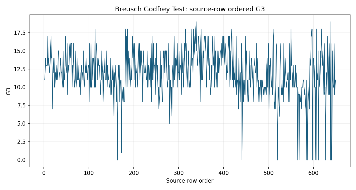
Python chart 1: Breusch Godfrey Test
The Python figure for Breusch Godfrey Test presents the source series and time ordering. Its file name is breusch godfrey test 01 source series. Interpret this chart with the worked statistics and the matching Python PDF; the image alone does not establish the final inference.
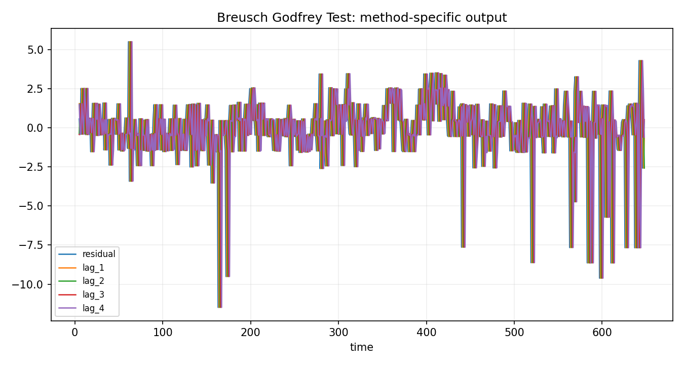
Python chart 2: Breusch Godfrey Test
The Python figure for Breusch Godfrey Test presents the method-specific fitted or transformed output. Its file name is breusch godfrey test 02 method output. Interpret this chart with the worked statistics and the matching Python PDF; the image alone does not establish the final inference.
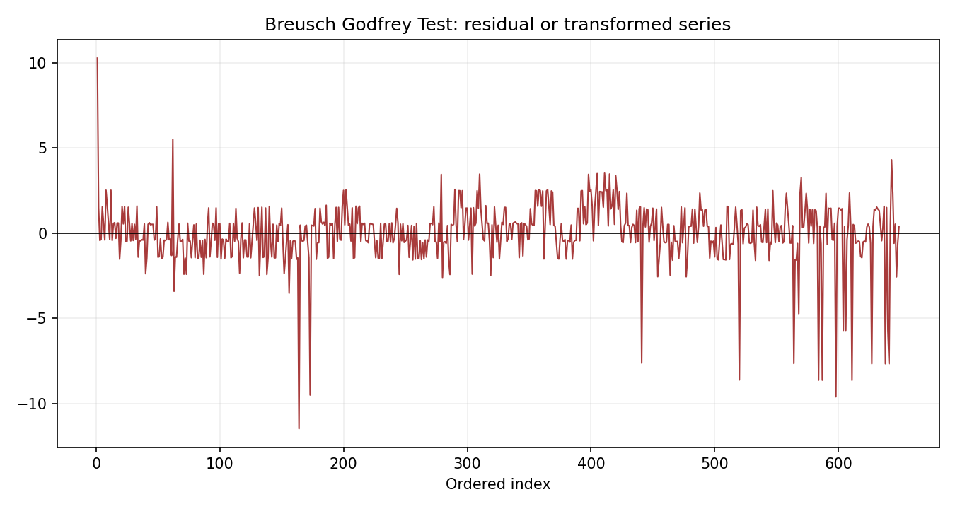
Python chart 3: Breusch Godfrey Test
The Python figure for Breusch Godfrey Test presents the residual path through time. Its file name is breusch godfrey test 03 residual path. Interpret this chart with the worked statistics and the matching Python PDF; the image alone does not establish the final inference.
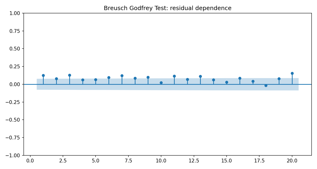
Python chart 4: Breusch Godfrey Test
The Python figure for Breusch Godfrey Test presents the residual autocorrelation diagnostics. Its file name is breusch godfrey test 04 residual acf. Interpret this chart with the worked statistics and the matching Python PDF; the image alone does not establish the final inference.
Breusch Godfrey Test in R
Equivalent specification with explicit frequency.
# Regress residuals on original regressors and 12 lagged residuals; use n*R^2.The R workflow must use the same start date, frequency, training endpoint, lag order, deterministic structure, and forecast horizon. Reconcile default initialization, missing-value behavior, coefficient signs, and critical values before comparing numerical output with Python.
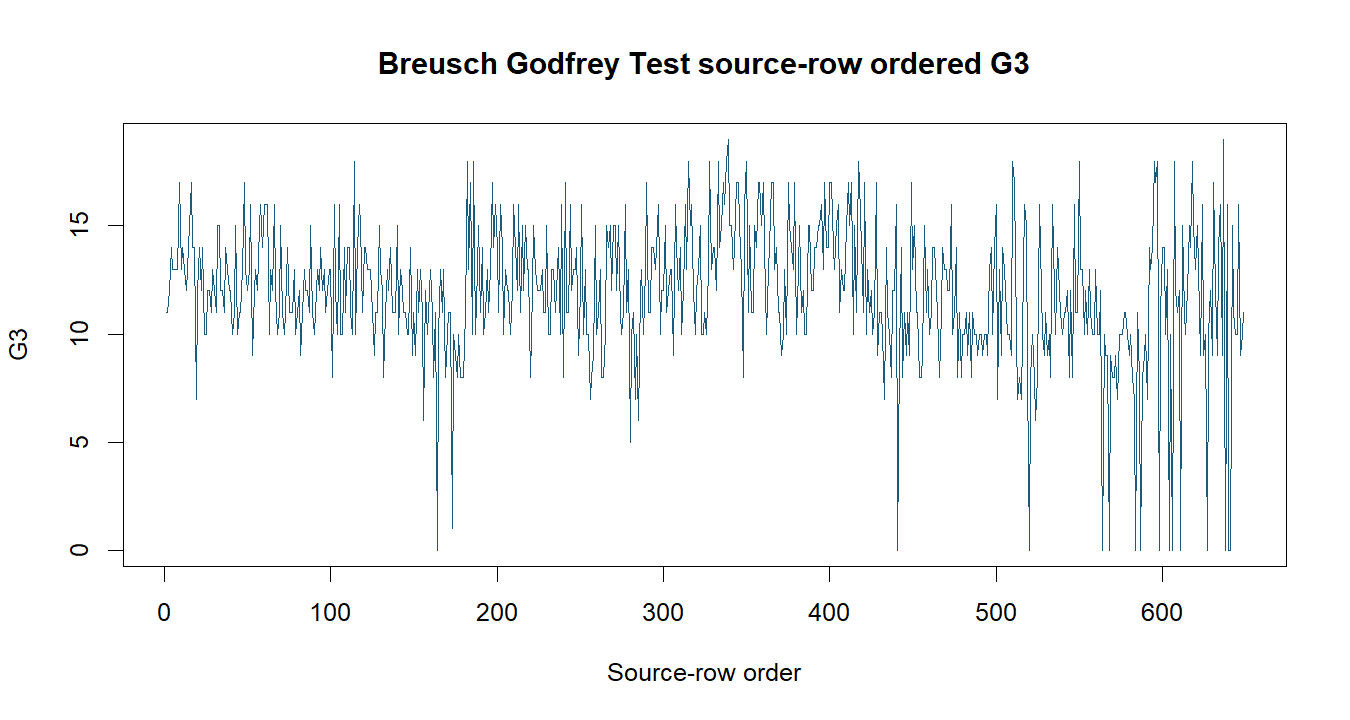
R chart 1: Breusch Godfrey Test
The R figure for Breusch Godfrey Test presents the source series and time ordering. Its file name is breusch godfrey test 01. Interpret this chart with the worked statistics and the matching R PDF; the image alone does not establish the final inference.
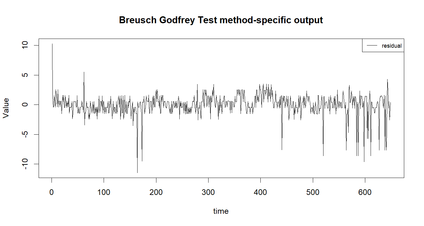
R chart 2: Breusch Godfrey Test
The R figure for Breusch Godfrey Test presents the method-specific fitted or transformed output. Its file name is breusch godfrey test 02. Interpret this chart with the worked statistics and the matching R PDF; the image alone does not establish the final inference.
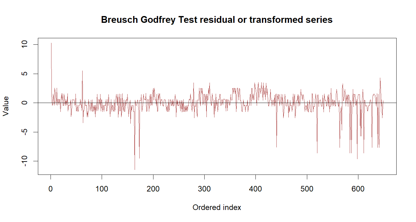
R chart 3: Breusch Godfrey Test
The R figure for Breusch Godfrey Test presents the residual path through time. Its file name is breusch godfrey test 03. Interpret this chart with the worked statistics and the matching R PDF; the image alone does not establish the final inference.
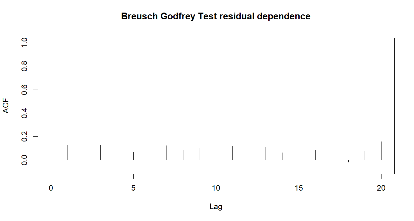
R chart 4: Breusch Godfrey Test
The R figure for Breusch Godfrey Test presents the residual autocorrelation diagnostics. Its file name is breusch godfrey test 04. Interpret this chart with the worked statistics and the matching R PDF; the image alone does not establish the final inference.
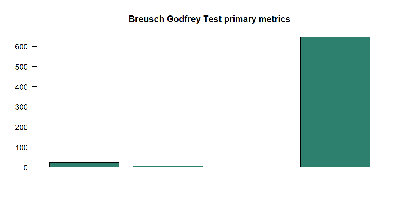
R chart 5: Breusch Godfrey Test
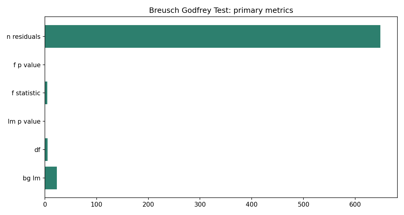
The R figure for Breusch Godfrey Test presents the primary statistics and validation metrics. Its file name is breusch godfrey test 05. Interpret this chart with the worked statistics and the matching R PDF; the image alone does not establish the final inference.
Breusch Godfrey Test in SPSS
Use only procedures SPSS genuinely supports.
Use Analyze > Forecasting > Autocorrelations for ACF/PACF and save model residuals before residual diagnostics. For regression-based diagnostics, create lagged residual variables and keep the original regressors in the auxiliary equation.
Breusch Godfrey Test in Excel
A transparent formula and range audit.
Fit the original regression and retain residuals. Regress the residuals on the same original regressors together with q lagged residuals, using the same valid rows after lag construction. Calculate LM = n_valid * R_squared from this auxiliary regression and compare with a chi-square distribution with q degrees of freedom under appropriate asymptotic conditions; alternatively use the auxiliary regression’s joint F test. An ACF-only correlation calculation or Box–Pierce/Ljung–Box Q statistic is not the Breusch–Godfrey test.
How to interpret Breusch Godfrey Test charts
Each chart has a distinct technical role.
Source or input chart
Check order, missing periods, changing level, seasonality, outliers, and possible breaks before fitting. A visually attractive series is not automatically stationary or forecastable.
Method-output chart
Compare fitted and observed behavior or the method-specific transformation. Look for systematic misses, phase errors, and delayed responses rather than only visual closeness.
Residual and metric charts
Residual paths and autocorrelation show what predictable structure remains. Metric panels summarize holdout performance but must retain the horizon and units.
Breusch Godfrey Test diagnostics and failure checks
Evidence that the result is usable.
Deep technical review of Breusch Godfrey Test
Forty-eight topic-specific audit perspectives.
Temporal order. For Breusch Godfrey Test, this review point concerns why the sequence must remain chronological and how random shuffling would leak future information. The method specifically tests higher-order residual serial correlation in a regression while accommodating lagged dependent variables and other regressors; therefore the analyst should connect this issue to the distinction between raw-series and residual dependence, lag-specific coefficients, and joint portmanteau evidence. In the worked example, The Breusch–Godfrey LM statistic was 77.529 with p < .001, indicating residual record-order correlation through 12 lags. That numerical result is useful only when the date index, training endpoint, and declared frequency remain unchanged. A defensible audit records the choice before seeing the final forecast error or p-value, checks the matching chart and software output, and explains whether the conclusion would change under a reasonable alternative. Related guidance appears in Autocorrelation Function, Partial Autocorrelation Function, Box Pierce Test, but those methods answer different parts of the identification, estimation, diagnostic, or validation problem.
Frequency declaration. For Breusch Godfrey Test, this review point concerns how monthly, quarterly, daily, or irregular spacing changes lag meaning and seasonal interpretation. The method specifically tests higher-order residual serial correlation in a regression while accommodating lagged dependent variables and other regressors; therefore the analyst should connect this issue to the distinction between raw-series and residual dependence, lag-specific coefficients, and joint portmanteau evidence. In the worked example, The Breusch–Godfrey LM statistic was 77.529 with p < .001, indicating residual record-order correlation through 12 lags. That numerical result is useful only when the date index, training endpoint, and declared frequency remain unchanged. A defensible audit records the choice before seeing the final forecast error or p-value, checks the matching chart and software output, and explains whether the conclusion would change under a reasonable alternative. Related guidance appears in Autocorrelation Function, Partial Autocorrelation Function, Box Pierce Test, but those methods answer different parts of the identification, estimation, diagnostic, or validation problem.
Missing periods. For Breusch Godfrey Test, this review point concerns how absent timestamps differ from observed zero values and how each should be represented. The method specifically tests higher-order residual serial correlation in a regression while accommodating lagged dependent variables and other regressors; therefore the analyst should connect this issue to the distinction between raw-series and residual dependence, lag-specific coefficients, and joint portmanteau evidence. In the worked example, The Breusch–Godfrey LM statistic was 77.529 with p < .001, indicating residual record-order correlation through 12 lags. That numerical result is useful only when the date index, training endpoint, and declared frequency remain unchanged. A defensible audit records the choice before seeing the final forecast error or p-value, checks the matching chart and software output, and explains whether the conclusion would change under a reasonable alternative. Related guidance appears in Autocorrelation Function, Partial Autocorrelation Function, Box Pierce Test, but those methods answer different parts of the identification, estimation, diagnostic, or validation problem.
Duplicate timestamps. For Breusch Godfrey Test, this review point concerns how multiple records at one time point require an explicit aggregation or disaggregation rule. The method specifically tests higher-order residual serial correlation in a regression while accommodating lagged dependent variables and other regressors; therefore the analyst should connect this issue to the distinction between raw-series and residual dependence, lag-specific coefficients, and joint portmanteau evidence. In the worked example, The Breusch–Godfrey LM statistic was 77.529 with p < .001, indicating residual record-order correlation through 12 lags. That numerical result is useful only when the date index, training endpoint, and declared frequency remain unchanged. A defensible audit records the choice before seeing the final forecast error or p-value, checks the matching chart and software output, and explains whether the conclusion would change under a reasonable alternative. Related guidance appears in Autocorrelation Function, Partial Autocorrelation Function, Box Pierce Test, but those methods answer different parts of the identification, estimation, diagnostic, or validation problem.
Units and scaling. For Breusch Godfrey Test, this review point concerns how coefficients and error summaries inherit the outcome scale and how transformations alter interpretation. The method specifically tests higher-order residual serial correlation in a regression while accommodating lagged dependent variables and other regressors; therefore the analyst should connect this issue to the distinction between raw-series and residual dependence, lag-specific coefficients, and joint portmanteau evidence. In the worked example, The Breusch–Godfrey LM statistic was 77.529 with p < .001, indicating residual record-order correlation through 12 lags. That numerical result is useful only when the date index, training endpoint, and declared frequency remain unchanged. A defensible audit records the choice before seeing the final forecast error or p-value, checks the matching chart and software output, and explains whether the conclusion would change under a reasonable alternative. Related guidance appears in Autocorrelation Function, Partial Autocorrelation Function, Box Pierce Test, but those methods answer different parts of the identification, estimation, diagnostic, or validation problem.
Log transformation. For Breusch Godfrey Test, this review point concerns when multiplicative growth or variance stabilization supports a log scale and when zeros make it unsuitable. The method specifically tests higher-order residual serial correlation in a regression while accommodating lagged dependent variables and other regressors; therefore the analyst should connect this issue to the distinction between raw-series and residual dependence, lag-specific coefficients, and joint portmanteau evidence. In the worked example, The Breusch–Godfrey LM statistic was 77.529 with p < .001, indicating residual record-order correlation through 12 lags. That numerical result is useful only when the date index, training endpoint, and declared frequency remain unchanged. A defensible audit records the choice before seeing the final forecast error or p-value, checks the matching chart and software output, and explains whether the conclusion would change under a reasonable alternative. Related guidance appears in Autocorrelation Function, Partial Autocorrelation Function, Box Pierce Test, but those methods answer different parts of the identification, estimation, diagnostic, or validation problem.
Differencing. For Breusch Godfrey Test, this review point concerns how regular and seasonal differences remove stochastic trends but also change the target being modeled. The method specifically tests higher-order residual serial correlation in a regression while accommodating lagged dependent variables and other regressors; therefore the analyst should connect this issue to the distinction between raw-series and residual dependence, lag-specific coefficients, and joint portmanteau evidence. In the worked example, The Breusch–Godfrey LM statistic was 77.529 with p < .001, indicating residual record-order correlation through 12 lags. That numerical result is useful only when the date index, training endpoint, and declared frequency remain unchanged. A defensible audit records the choice before seeing the final forecast error or p-value, checks the matching chart and software output, and explains whether the conclusion would change under a reasonable alternative. Related guidance appears in Autocorrelation Function, Partial Autocorrelation Function, Box Pierce Test, but those methods answer different parts of the identification, estimation, diagnostic, or validation problem.
Deterministic trend. For Breusch Godfrey Test, this review point concerns why an intercept, time trend, or seasonal dummies must reflect the scientific specification. The method specifically tests higher-order residual serial correlation in a regression while accommodating lagged dependent variables and other regressors; therefore the analyst should connect this issue to the distinction between raw-series and residual dependence, lag-specific coefficients, and joint portmanteau evidence. In the worked example, The Breusch–Godfrey LM statistic was 77.529 with p < .001, indicating residual record-order correlation through 12 lags. That numerical result is useful only when the date index, training endpoint, and declared frequency remain unchanged. A defensible audit records the choice before seeing the final forecast error or p-value, checks the matching chart and software output, and explains whether the conclusion would change under a reasonable alternative. Related guidance appears in Autocorrelation Function, Partial Autocorrelation Function, Box Pierce Test, but those methods answer different parts of the identification, estimation, diagnostic, or validation problem.
Seasonal period. For Breusch Godfrey Test, this review point concerns how a period of 12 for monthly data differs from a vague visual cycle and must be declared before estimation. The method specifically tests higher-order residual serial correlation in a regression while accommodating lagged dependent variables and other regressors; therefore the analyst should connect this issue to the distinction between raw-series and residual dependence, lag-specific coefficients, and joint portmanteau evidence. In the worked example, The Breusch–Godfrey LM statistic was 77.529 with p < .001, indicating residual record-order correlation through 12 lags. That numerical result is useful only when the date index, training endpoint, and declared frequency remain unchanged. A defensible audit records the choice before seeing the final forecast error or p-value, checks the matching chart and software output, and explains whether the conclusion would change under a reasonable alternative. Related guidance appears in Autocorrelation Function, Partial Autocorrelation Function, Box Pierce Test, but those methods answer different parts of the identification, estimation, diagnostic, or validation problem.
Lag order. For Breusch Godfrey Test, this review point concerns how information criteria, domain timing, residual diagnostics, and sample size jointly constrain lag selection. The method specifically tests higher-order residual serial correlation in a regression while accommodating lagged dependent variables and other regressors; therefore the analyst should connect this issue to the distinction between raw-series and residual dependence, lag-specific coefficients, and joint portmanteau evidence. In the worked example, The Breusch–Godfrey LM statistic was 77.529 with p < .001, indicating residual record-order correlation through 12 lags. That numerical result is useful only when the date index, training endpoint, and declared frequency remain unchanged. A defensible audit records the choice before seeing the final forecast error or p-value, checks the matching chart and software output, and explains whether the conclusion would change under a reasonable alternative. Related guidance appears in Autocorrelation Function, Partial Autocorrelation Function, Box Pierce Test, but those methods answer different parts of the identification, estimation, diagnostic, or validation problem.
Parameter signs. For Breusch Godfrey Test, this review point concerns how positive and negative coefficients affect persistence, correction, oscillation, or response direction. The method specifically tests higher-order residual serial correlation in a regression while accommodating lagged dependent variables and other regressors; therefore the analyst should connect this issue to the distinction between raw-series and residual dependence, lag-specific coefficients, and joint portmanteau evidence. In the worked example, The Breusch–Godfrey LM statistic was 77.529 with p < .001, indicating residual record-order correlation through 12 lags. That numerical result is useful only when the date index, training endpoint, and declared frequency remain unchanged. A defensible audit records the choice before seeing the final forecast error or p-value, checks the matching chart and software output, and explains whether the conclusion would change under a reasonable alternative. Related guidance appears in Autocorrelation Function, Partial Autocorrelation Function, Box Pierce Test, but those methods answer different parts of the identification, estimation, diagnostic, or validation problem.
Parameter magnitude. For Breusch Godfrey Test, this review point concerns why a numerically large coefficient is not automatically important without considering the full dynamic polynomial. The method specifically tests higher-order residual serial correlation in a regression while accommodating lagged dependent variables and other regressors; therefore the analyst should connect this issue to the distinction between raw-series and residual dependence, lag-specific coefficients, and joint portmanteau evidence. In the worked example, The Breusch–Godfrey LM statistic was 77.529 with p < .001, indicating residual record-order correlation through 12 lags. That numerical result is useful only when the date index, training endpoint, and declared frequency remain unchanged. A defensible audit records the choice before seeing the final forecast error or p-value, checks the matching chart and software output, and explains whether the conclusion would change under a reasonable alternative. Related guidance appears in Autocorrelation Function, Partial Autocorrelation Function, Box Pierce Test, but those methods answer different parts of the identification, estimation, diagnostic, or validation problem.
Model admissibility. For Breusch Godfrey Test, this review point concerns how stationarity, invertibility, positivity, or rank restrictions protect the mathematical process. The method specifically tests higher-order residual serial correlation in a regression while accommodating lagged dependent variables and other regressors; therefore the analyst should connect this issue to the distinction between raw-series and residual dependence, lag-specific coefficients, and joint portmanteau evidence. In the worked example, The Breusch–Godfrey LM statistic was 77.529 with p < .001, indicating residual record-order correlation through 12 lags. That numerical result is useful only when the date index, training endpoint, and declared frequency remain unchanged. A defensible audit records the choice before seeing the final forecast error or p-value, checks the matching chart and software output, and explains whether the conclusion would change under a reasonable alternative. Related guidance appears in Autocorrelation Function, Partial Autocorrelation Function, Box Pierce Test, but those methods answer different parts of the identification, estimation, diagnostic, or validation problem.
Initial conditions. For Breusch Godfrey Test, this review point concerns how early state values or unavailable lags influence fitting and why software defaults should be recorded. The method specifically tests higher-order residual serial correlation in a regression while accommodating lagged dependent variables and other regressors; therefore the analyst should connect this issue to the distinction between raw-series and residual dependence, lag-specific coefficients, and joint portmanteau evidence. In the worked example, The Breusch–Godfrey LM statistic was 77.529 with p < .001, indicating residual record-order correlation through 12 lags. That numerical result is useful only when the date index, training endpoint, and declared frequency remain unchanged. A defensible audit records the choice before seeing the final forecast error or p-value, checks the matching chart and software output, and explains whether the conclusion would change under a reasonable alternative. Related guidance appears in Autocorrelation Function, Partial Autocorrelation Function, Box Pierce Test, but those methods answer different parts of the identification, estimation, diagnostic, or validation problem.
Optimization convergence. For Breusch Godfrey Test, this review point concerns how a returned result can still be unreliable when the likelihood optimizer stops at a boundary or local solution. The method specifically tests higher-order residual serial correlation in a regression while accommodating lagged dependent variables and other regressors; therefore the analyst should connect this issue to the distinction between raw-series and residual dependence, lag-specific coefficients, and joint portmanteau evidence. In the worked example, The Breusch–Godfrey LM statistic was 77.529 with p < .001, indicating residual record-order correlation through 12 lags. That numerical result is useful only when the date index, training endpoint, and declared frequency remain unchanged. A defensible audit records the choice before seeing the final forecast error or p-value, checks the matching chart and software output, and explains whether the conclusion would change under a reasonable alternative. Related guidance appears in Autocorrelation Function, Partial Autocorrelation Function, Box Pierce Test, but those methods answer different parts of the identification, estimation, diagnostic, or validation problem.
Residual mean. For Breusch Godfrey Test, this review point concerns why systematic residual bias indicates an omitted level, trend, transformation, or deterministic component. The method specifically tests higher-order residual serial correlation in a regression while accommodating lagged dependent variables and other regressors; therefore the analyst should connect this issue to the distinction between raw-series and residual dependence, lag-specific coefficients, and joint portmanteau evidence. In the worked example, The Breusch–Godfrey LM statistic was 77.529 with p < .001, indicating residual record-order correlation through 12 lags. That numerical result is useful only when the date index, training endpoint, and declared frequency remain unchanged. A defensible audit records the choice before seeing the final forecast error or p-value, checks the matching chart and software output, and explains whether the conclusion would change under a reasonable alternative. Related guidance appears in Autocorrelation Function, Partial Autocorrelation Function, Box Pierce Test, but those methods answer different parts of the identification, estimation, diagnostic, or validation problem.
Residual autocorrelation. For Breusch Godfrey Test, this review point concerns why remaining serial structure means the model has not extracted all predictable timing information. The method specifically tests higher-order residual serial correlation in a regression while accommodating lagged dependent variables and other regressors; therefore the analyst should connect this issue to the distinction between raw-series and residual dependence, lag-specific coefficients, and joint portmanteau evidence. In the worked example, The Breusch–Godfrey LM statistic was 77.529 with p < .001, indicating residual record-order correlation through 12 lags. That numerical result is useful only when the date index, training endpoint, and declared frequency remain unchanged. A defensible audit records the choice before seeing the final forecast error or p-value, checks the matching chart and software output, and explains whether the conclusion would change under a reasonable alternative. Related guidance appears in Autocorrelation Function, Partial Autocorrelation Function, Box Pierce Test, but those methods answer different parts of the identification, estimation, diagnostic, or validation problem.
Residual variance. For Breusch Godfrey Test, this review point concerns how changing error spread affects standard errors, intervals, and the relative value of volatility models. The method specifically tests higher-order residual serial correlation in a regression while accommodating lagged dependent variables and other regressors; therefore the analyst should connect this issue to the distinction between raw-series and residual dependence, lag-specific coefficients, and joint portmanteau evidence. In the worked example, The Breusch–Godfrey LM statistic was 77.529 with p < .001, indicating residual record-order correlation through 12 lags. That numerical result is useful only when the date index, training endpoint, and declared frequency remain unchanged. A defensible audit records the choice before seeing the final forecast error or p-value, checks the matching chart and software output, and explains whether the conclusion would change under a reasonable alternative. Related guidance appears in Autocorrelation Function, Partial Autocorrelation Function, Box Pierce Test, but those methods answer different parts of the identification, estimation, diagnostic, or validation problem.
Residual distribution. For Breusch Godfrey Test, this review point concerns why heavy tails and outliers can make normal-based intervals too narrow even when point forecasts look reasonable. The method specifically tests higher-order residual serial correlation in a regression while accommodating lagged dependent variables and other regressors; therefore the analyst should connect this issue to the distinction between raw-series and residual dependence, lag-specific coefficients, and joint portmanteau evidence. In the worked example, The Breusch–Godfrey LM statistic was 77.529 with p < .001, indicating residual record-order correlation through 12 lags. That numerical result is useful only when the date index, training endpoint, and declared frequency remain unchanged. A defensible audit records the choice before seeing the final forecast error or p-value, checks the matching chart and software output, and explains whether the conclusion would change under a reasonable alternative. Related guidance appears in Autocorrelation Function, Partial Autocorrelation Function, Box Pierce Test, but those methods answer different parts of the identification, estimation, diagnostic, or validation problem.
Outlier timing. For Breusch Godfrey Test, this review point concerns how isolated shocks, additive outliers, and level shifts require different interpretations and interventions. The method specifically tests higher-order residual serial correlation in a regression while accommodating lagged dependent variables and other regressors; therefore the analyst should connect this issue to the distinction between raw-series and residual dependence, lag-specific coefficients, and joint portmanteau evidence. In the worked example, The Breusch–Godfrey LM statistic was 77.529 with p < .001, indicating residual record-order correlation through 12 lags. That numerical result is useful only when the date index, training endpoint, and declared frequency remain unchanged. A defensible audit records the choice before seeing the final forecast error or p-value, checks the matching chart and software output, and explains whether the conclusion would change under a reasonable alternative. Related guidance appears in Autocorrelation Function, Partial Autocorrelation Function, Box Pierce Test, but those methods answer different parts of the identification, estimation, diagnostic, or validation problem.
Structural breaks. For Breusch Godfrey Test, this review point concerns how policy, measurement, market, or operational changes can invalidate a single stable-parameter model. The method specifically tests higher-order residual serial correlation in a regression while accommodating lagged dependent variables and other regressors; therefore the analyst should connect this issue to the distinction between raw-series and residual dependence, lag-specific coefficients, and joint portmanteau evidence. In the worked example, The Breusch–Godfrey LM statistic was 77.529 with p < .001, indicating residual record-order correlation through 12 lags. That numerical result is useful only when the date index, training endpoint, and declared frequency remain unchanged. A defensible audit records the choice before seeing the final forecast error or p-value, checks the matching chart and software output, and explains whether the conclusion would change under a reasonable alternative. Related guidance appears in Autocorrelation Function, Partial Autocorrelation Function, Box Pierce Test, but those methods answer different parts of the identification, estimation, diagnostic, or validation problem.
Training endpoint. For Breusch Godfrey Test, this review point concerns why every tuning choice must use observations available at or before the declared forecast origin. The method specifically tests higher-order residual serial correlation in a regression while accommodating lagged dependent variables and other regressors; therefore the analyst should connect this issue to the distinction between raw-series and residual dependence, lag-specific coefficients, and joint portmanteau evidence. In the worked example, The Breusch–Godfrey LM statistic was 77.529 with p < .001, indicating residual record-order correlation through 12 lags. That numerical result is useful only when the date index, training endpoint, and declared frequency remain unchanged. A defensible audit records the choice before seeing the final forecast error or p-value, checks the matching chart and software output, and explains whether the conclusion would change under a reasonable alternative. Related guidance appears in Autocorrelation Function, Partial Autocorrelation Function, Box Pierce Test, but those methods answer different parts of the identification, estimation, diagnostic, or validation problem.
Holdout horizon. For Breusch Godfrey Test, this review point concerns how one-step and twelve-step performance answer different operational forecasting questions. The method specifically tests higher-order residual serial correlation in a regression while accommodating lagged dependent variables and other regressors; therefore the analyst should connect this issue to the distinction between raw-series and residual dependence, lag-specific coefficients, and joint portmanteau evidence. In the worked example, The Breusch–Godfrey LM statistic was 77.529 with p < .001, indicating residual record-order correlation through 12 lags. That numerical result is useful only when the date index, training endpoint, and declared frequency remain unchanged. A defensible audit records the choice before seeing the final forecast error or p-value, checks the matching chart and software output, and explains whether the conclusion would change under a reasonable alternative. Related guidance appears in Autocorrelation Function, Partial Autocorrelation Function, Box Pierce Test, but those methods answer different parts of the identification, estimation, diagnostic, or validation problem.
Rolling-origin validation. For Breusch Godfrey Test, this review point concerns how repeated forecast origins reveal whether one favorable split is representative. The method specifically tests higher-order residual serial correlation in a regression while accommodating lagged dependent variables and other regressors; therefore the analyst should connect this issue to the distinction between raw-series and residual dependence, lag-specific coefficients, and joint portmanteau evidence. In the worked example, The Breusch–Godfrey LM statistic was 77.529 with p < .001, indicating residual record-order correlation through 12 lags. That numerical result is useful only when the date index, training endpoint, and declared frequency remain unchanged. A defensible audit records the choice before seeing the final forecast error or p-value, checks the matching chart and software output, and explains whether the conclusion would change under a reasonable alternative. Related guidance appears in Autocorrelation Function, Partial Autocorrelation Function, Box Pierce Test, but those methods answer different parts of the identification, estimation, diagnostic, or validation problem.
Baseline comparison. For Breusch Godfrey Test, this review point concerns why a naive, seasonal-naive, or simple smoothing forecast is needed before claiming improvement. The method specifically tests higher-order residual serial correlation in a regression while accommodating lagged dependent variables and other regressors; therefore the analyst should connect this issue to the distinction between raw-series and residual dependence, lag-specific coefficients, and joint portmanteau evidence. In the worked example, The Breusch–Godfrey LM statistic was 77.529 with p < .001, indicating residual record-order correlation through 12 lags. That numerical result is useful only when the date index, training endpoint, and declared frequency remain unchanged. A defensible audit records the choice before seeing the final forecast error or p-value, checks the matching chart and software output, and explains whether the conclusion would change under a reasonable alternative. Related guidance appears in Autocorrelation Function, Partial Autocorrelation Function, Box Pierce Test, but those methods answer different parts of the identification, estimation, diagnostic, or validation problem.
Metric selection. For Breusch Godfrey Test, this review point concerns how MAE, RMSE, MAPE, information criteria, and statistical tests answer different questions. The method specifically tests higher-order residual serial correlation in a regression while accommodating lagged dependent variables and other regressors; therefore the analyst should connect this issue to the distinction between raw-series and residual dependence, lag-specific coefficients, and joint portmanteau evidence. In the worked example, The Breusch–Godfrey LM statistic was 77.529 with p < .001, indicating residual record-order correlation through 12 lags. That numerical result is useful only when the date index, training endpoint, and declared frequency remain unchanged. A defensible audit records the choice before seeing the final forecast error or p-value, checks the matching chart and software output, and explains whether the conclusion would change under a reasonable alternative. Related guidance appears in Autocorrelation Function, Partial Autocorrelation Function, Box Pierce Test, but those methods answer different parts of the identification, estimation, diagnostic, or validation problem.
Forecast intervals. For Breusch Godfrey Test, this review point concerns why uncertainty should widen with horizon and why point accuracy alone is incomplete. The method specifically tests higher-order residual serial correlation in a regression while accommodating lagged dependent variables and other regressors; therefore the analyst should connect this issue to the distinction between raw-series and residual dependence, lag-specific coefficients, and joint portmanteau evidence. In the worked example, The Breusch–Godfrey LM statistic was 77.529 with p < .001, indicating residual record-order correlation through 12 lags. That numerical result is useful only when the date index, training endpoint, and declared frequency remain unchanged. A defensible audit records the choice before seeing the final forecast error or p-value, checks the matching chart and software output, and explains whether the conclusion would change under a reasonable alternative. Related guidance appears in Autocorrelation Function, Partial Autocorrelation Function, Box Pierce Test, but those methods answer different parts of the identification, estimation, diagnostic, or validation problem.
Small samples. For Breusch Godfrey Test, this review point concerns how parameter count, lag loss, and unstable asymptotics become especially important with short histories. The method specifically tests higher-order residual serial correlation in a regression while accommodating lagged dependent variables and other regressors; therefore the analyst should connect this issue to the distinction between raw-series and residual dependence, lag-specific coefficients, and joint portmanteau evidence. In the worked example, The Breusch–Godfrey LM statistic was 77.529 with p < .001, indicating residual record-order correlation through 12 lags. That numerical result is useful only when the date index, training endpoint, and declared frequency remain unchanged. A defensible audit records the choice before seeing the final forecast error or p-value, checks the matching chart and software output, and explains whether the conclusion would change under a reasonable alternative. Related guidance appears in Autocorrelation Function, Partial Autocorrelation Function, Box Pierce Test, but those methods answer different parts of the identification, estimation, diagnostic, or validation problem.
Large samples. For Breusch Godfrey Test, this review point concerns why tiny p-values can coexist with operationally negligible effects and why diagnostics still matter. The method specifically tests higher-order residual serial correlation in a regression while accommodating lagged dependent variables and other regressors; therefore the analyst should connect this issue to the distinction between raw-series and residual dependence, lag-specific coefficients, and joint portmanteau evidence. In the worked example, The Breusch–Godfrey LM statistic was 77.529 with p < .001, indicating residual record-order correlation through 12 lags. That numerical result is useful only when the date index, training endpoint, and declared frequency remain unchanged. A defensible audit records the choice before seeing the final forecast error or p-value, checks the matching chart and software output, and explains whether the conclusion would change under a reasonable alternative. Related guidance appears in Autocorrelation Function, Partial Autocorrelation Function, Box Pierce Test, but those methods answer different parts of the identification, estimation, diagnostic, or validation problem.
Multiple series. For Breusch Godfrey Test, this review point concerns how comparing or combining series requires aligned calendars and consistent transformations. The method specifically tests higher-order residual serial correlation in a regression while accommodating lagged dependent variables and other regressors; therefore the analyst should connect this issue to the distinction between raw-series and residual dependence, lag-specific coefficients, and joint portmanteau evidence. In the worked example, The Breusch–Godfrey LM statistic was 77.529 with p < .001, indicating residual record-order correlation through 12 lags. That numerical result is useful only when the date index, training endpoint, and declared frequency remain unchanged. A defensible audit records the choice before seeing the final forecast error or p-value, checks the matching chart and software output, and explains whether the conclusion would change under a reasonable alternative. Related guidance appears in Autocorrelation Function, Partial Autocorrelation Function, Box Pierce Test, but those methods answer different parts of the identification, estimation, diagnostic, or validation problem.
Exogenous variables. For Breusch Godfrey Test, this review point concerns how external predictors must be known or forecast at future horizons to support genuine forecasts. The method specifically tests higher-order residual serial correlation in a regression while accommodating lagged dependent variables and other regressors; therefore the analyst should connect this issue to the distinction between raw-series and residual dependence, lag-specific coefficients, and joint portmanteau evidence. In the worked example, The Breusch–Godfrey LM statistic was 77.529 with p < .001, indicating residual record-order correlation through 12 lags. That numerical result is useful only when the date index, training endpoint, and declared frequency remain unchanged. A defensible audit records the choice before seeing the final forecast error or p-value, checks the matching chart and software output, and explains whether the conclusion would change under a reasonable alternative. Related guidance appears in Autocorrelation Function, Partial Autocorrelation Function, Box Pierce Test, but those methods answer different parts of the identification, estimation, diagnostic, or validation problem.
Data leakage. For Breusch Godfrey Test, this review point concerns how centered moving averages, full-sample scaling, or future-informed imputation can contaminate validation. The method specifically tests higher-order residual serial correlation in a regression while accommodating lagged dependent variables and other regressors; therefore the analyst should connect this issue to the distinction between raw-series and residual dependence, lag-specific coefficients, and joint portmanteau evidence. In the worked example, The Breusch–Godfrey LM statistic was 77.529 with p < .001, indicating residual record-order correlation through 12 lags. That numerical result is useful only when the date index, training endpoint, and declared frequency remain unchanged. A defensible audit records the choice before seeing the final forecast error or p-value, checks the matching chart and software output, and explains whether the conclusion would change under a reasonable alternative. Related guidance appears in Autocorrelation Function, Partial Autocorrelation Function, Box Pierce Test, but those methods answer different parts of the identification, estimation, diagnostic, or validation problem.
Software defaults. For Breusch Godfrey Test, this review point concerns why default trends, lag selection, missing-value handling, and parameter signs can differ across programs. The method specifically tests higher-order residual serial correlation in a regression while accommodating lagged dependent variables and other regressors; therefore the analyst should connect this issue to the distinction between raw-series and residual dependence, lag-specific coefficients, and joint portmanteau evidence. In the worked example, The Breusch–Godfrey LM statistic was 77.529 with p < .001, indicating residual record-order correlation through 12 lags. That numerical result is useful only when the date index, training endpoint, and declared frequency remain unchanged. A defensible audit records the choice before seeing the final forecast error or p-value, checks the matching chart and software output, and explains whether the conclusion would change under a reasonable alternative. Related guidance appears in Autocorrelation Function, Partial Autocorrelation Function, Box Pierce Test, but those methods answer different parts of the identification, estimation, diagnostic, or validation problem.
Numerical precision. For Breusch Godfrey Test, this review point concerns why displayed rounding should not replace full-precision calculations or reconciliation tables. The method specifically tests higher-order residual serial correlation in a regression while accommodating lagged dependent variables and other regressors; therefore the analyst should connect this issue to the distinction between raw-series and residual dependence, lag-specific coefficients, and joint portmanteau evidence. In the worked example, The Breusch–Godfrey LM statistic was 77.529 with p < .001, indicating residual record-order correlation through 12 lags. That numerical result is useful only when the date index, training endpoint, and declared frequency remain unchanged. A defensible audit records the choice before seeing the final forecast error or p-value, checks the matching chart and software output, and explains whether the conclusion would change under a reasonable alternative. Related guidance appears in Autocorrelation Function, Partial Autocorrelation Function, Box Pierce Test, but those methods answer different parts of the identification, estimation, diagnostic, or validation problem.
Chart interpretation. For Breusch Godfrey Test, this review point concerns how the source-series, fitted-output, residual-path, residual-ACF, and metric charts answer different questions. The method specifically tests higher-order residual serial correlation in a regression while accommodating lagged dependent variables and other regressors; therefore the analyst should connect this issue to the distinction between raw-series and residual dependence, lag-specific coefficients, and joint portmanteau evidence. In the worked example, The Breusch–Godfrey LM statistic was 77.529 with p < .001, indicating residual record-order correlation through 12 lags. That numerical result is useful only when the date index, training endpoint, and declared frequency remain unchanged. A defensible audit records the choice before seeing the final forecast error or p-value, checks the matching chart and software output, and explains whether the conclusion would change under a reasonable alternative. Related guidance appears in Autocorrelation Function, Partial Autocorrelation Function, Box Pierce Test, but those methods answer different parts of the identification, estimation, diagnostic, or validation problem.
Chart accessibility. For Breusch Godfrey Test, this review point concerns why meaningful alt text should state the variable, method, comparison, and visible conclusion. The method specifically tests higher-order residual serial correlation in a regression while accommodating lagged dependent variables and other regressors; therefore the analyst should connect this issue to the distinction between raw-series and residual dependence, lag-specific coefficients, and joint portmanteau evidence. In the worked example, The Breusch–Godfrey LM statistic was 77.529 with p < .001, indicating residual record-order correlation through 12 lags. That numerical result is useful only when the date index, training endpoint, and declared frequency remain unchanged. A defensible audit records the choice before seeing the final forecast error or p-value, checks the matching chart and software output, and explains whether the conclusion would change under a reasonable alternative. Related guidance appears in Autocorrelation Function, Partial Autocorrelation Function, Box Pierce Test, but those methods answer different parts of the identification, estimation, diagnostic, or validation problem.
Download integrity. For Breusch Godfrey Test, this review point concerns why each PDF and workbook must belong only to the matching topic and preserve the same sample and specification. The method specifically tests higher-order residual serial correlation in a regression while accommodating lagged dependent variables and other regressors; therefore the analyst should connect this issue to the distinction between raw-series and residual dependence, lag-specific coefficients, and joint portmanteau evidence. In the worked example, The Breusch–Godfrey LM statistic was 77.529 with p < .001, indicating residual record-order correlation through 12 lags. That numerical result is useful only when the date index, training endpoint, and declared frequency remain unchanged. A defensible audit records the choice before seeing the final forecast error or p-value, checks the matching chart and software output, and explains whether the conclusion would change under a reasonable alternative. Related guidance appears in Autocorrelation Function, Partial Autocorrelation Function, Box Pierce Test, but those methods answer different parts of the identification, estimation, diagnostic, or validation problem.
Reproducibility. For Breusch Godfrey Test, this review point concerns how a complete audit trail records data version, code version, random seed, specification, and exported results. The method specifically tests higher-order residual serial correlation in a regression while accommodating lagged dependent variables and other regressors; therefore the analyst should connect this issue to the distinction between raw-series and residual dependence, lag-specific coefficients, and joint portmanteau evidence. In the worked example, The Breusch–Godfrey LM statistic was 77.529 with p < .001, indicating residual record-order correlation through 12 lags. That numerical result is useful only when the date index, training endpoint, and declared frequency remain unchanged. A defensible audit records the choice before seeing the final forecast error or p-value, checks the matching chart and software output, and explains whether the conclusion would change under a reasonable alternative. Related guidance appears in Autocorrelation Function, Partial Autocorrelation Function, Box Pierce Test, but those methods answer different parts of the identification, estimation, diagnostic, or validation problem.
Decision language. For Breusch Godfrey Test, this review point concerns why fail-to-reject wording is different from proving a null model or exact equality. The method specifically tests higher-order residual serial correlation in a regression while accommodating lagged dependent variables and other regressors; therefore the analyst should connect this issue to the distinction between raw-series and residual dependence, lag-specific coefficients, and joint portmanteau evidence. In the worked example, The Breusch–Godfrey LM statistic was 77.529 with p < .001, indicating residual record-order correlation through 12 lags. That numerical result is useful only when the date index, training endpoint, and declared frequency remain unchanged. A defensible audit records the choice before seeing the final forecast error or p-value, checks the matching chart and software output, and explains whether the conclusion would change under a reasonable alternative. Related guidance appears in Autocorrelation Function, Partial Autocorrelation Function, Box Pierce Test, but those methods answer different parts of the identification, estimation, diagnostic, or validation problem.
Practical significance. For Breusch Godfrey Test, this review point concerns how statistical evidence must be connected to the size and consequence of the dynamic effect. The method specifically tests higher-order residual serial correlation in a regression while accommodating lagged dependent variables and other regressors; therefore the analyst should connect this issue to the distinction between raw-series and residual dependence, lag-specific coefficients, and joint portmanteau evidence. In the worked example, The Breusch–Godfrey LM statistic was 77.529 with p < .001, indicating residual record-order correlation through 12 lags. That numerical result is useful only when the date index, training endpoint, and declared frequency remain unchanged. A defensible audit records the choice before seeing the final forecast error or p-value, checks the matching chart and software output, and explains whether the conclusion would change under a reasonable alternative. Related guidance appears in Autocorrelation Function, Partial Autocorrelation Function, Box Pierce Test, but those methods answer different parts of the identification, estimation, diagnostic, or validation problem.
Sensitivity analysis. For Breusch Godfrey Test, this review point concerns how alternate lag orders, transformations, break dates, and seasonal periods test robustness. The method specifically tests higher-order residual serial correlation in a regression while accommodating lagged dependent variables and other regressors; therefore the analyst should connect this issue to the distinction between raw-series and residual dependence, lag-specific coefficients, and joint portmanteau evidence. In the worked example, The Breusch–Godfrey LM statistic was 77.529 with p < .001, indicating residual record-order correlation through 12 lags. That numerical result is useful only when the date index, training endpoint, and declared frequency remain unchanged. A defensible audit records the choice before seeing the final forecast error or p-value, checks the matching chart and software output, and explains whether the conclusion would change under a reasonable alternative. Related guidance appears in Autocorrelation Function, Partial Autocorrelation Function, Box Pierce Test, but those methods answer different parts of the identification, estimation, diagnostic, or validation problem.
Model parsimony. For Breusch Godfrey Test, this review point concerns why unnecessary parameters increase variance, complicate interpretation, and can worsen future performance. The method specifically tests higher-order residual serial correlation in a regression while accommodating lagged dependent variables and other regressors; therefore the analyst should connect this issue to the distinction between raw-series and residual dependence, lag-specific coefficients, and joint portmanteau evidence. In the worked example, The Breusch–Godfrey LM statistic was 77.529 with p < .001, indicating residual record-order correlation through 12 lags. That numerical result is useful only when the date index, training endpoint, and declared frequency remain unchanged. A defensible audit records the choice before seeing the final forecast error or p-value, checks the matching chart and software output, and explains whether the conclusion would change under a reasonable alternative. Related guidance appears in Autocorrelation Function, Partial Autocorrelation Function, Box Pierce Test, but those methods answer different parts of the identification, estimation, diagnostic, or validation problem.
Model underfit. For Breusch Godfrey Test, this review point concerns why a simple model can leave visible structure even when its in-sample error appears acceptable. The method specifically tests higher-order residual serial correlation in a regression while accommodating lagged dependent variables and other regressors; therefore the analyst should connect this issue to the distinction between raw-series and residual dependence, lag-specific coefficients, and joint portmanteau evidence. In the worked example, The Breusch–Godfrey LM statistic was 77.529 with p < .001, indicating residual record-order correlation through 12 lags. That numerical result is useful only when the date index, training endpoint, and declared frequency remain unchanged. A defensible audit records the choice before seeing the final forecast error or p-value, checks the matching chart and software output, and explains whether the conclusion would change under a reasonable alternative. Related guidance appears in Autocorrelation Function, Partial Autocorrelation Function, Box Pierce Test, but those methods answer different parts of the identification, estimation, diagnostic, or validation problem.
Model overfit. For Breusch Godfrey Test, this review point concerns why an elaborate model can absorb historical noise and fail at later forecast origins. The method specifically tests higher-order residual serial correlation in a regression while accommodating lagged dependent variables and other regressors; therefore the analyst should connect this issue to the distinction between raw-series and residual dependence, lag-specific coefficients, and joint portmanteau evidence. In the worked example, The Breusch–Godfrey LM statistic was 77.529 with p < .001, indicating residual record-order correlation through 12 lags. That numerical result is useful only when the date index, training endpoint, and declared frequency remain unchanged. A defensible audit records the choice before seeing the final forecast error or p-value, checks the matching chart and software output, and explains whether the conclusion would change under a reasonable alternative. Related guidance appears in Autocorrelation Function, Partial Autocorrelation Function, Box Pierce Test, but those methods answer different parts of the identification, estimation, diagnostic, or validation problem.
Documentation. For Breusch Godfrey Test, this review point concerns why the final report should state frequency, sample, transformations, lag orders, diagnostics, holdout design, and software. The method specifically tests higher-order residual serial correlation in a regression while accommodating lagged dependent variables and other regressors; therefore the analyst should connect this issue to the distinction between raw-series and residual dependence, lag-specific coefficients, and joint portmanteau evidence. In the worked example, The Breusch–Godfrey LM statistic was 77.529 with p < .001, indicating residual record-order correlation through 12 lags. That numerical result is useful only when the date index, training endpoint, and declared frequency remain unchanged. A defensible audit records the choice before seeing the final forecast error or p-value, checks the matching chart and software output, and explains whether the conclusion would change under a reasonable alternative. Related guidance appears in Autocorrelation Function, Partial Autocorrelation Function, Box Pierce Test, but those methods answer different parts of the identification, estimation, diagnostic, or validation problem.
Operational use. For Breusch Godfrey Test, this review point concerns how update frequency, retraining rules, monitoring thresholds, and fallback forecasts turn analysis into a maintainable process. The method specifically tests higher-order residual serial correlation in a regression while accommodating lagged dependent variables and other regressors; therefore the analyst should connect this issue to the distinction between raw-series and residual dependence, lag-specific coefficients, and joint portmanteau evidence. In the worked example, The Breusch–Godfrey LM statistic was 77.529 with p < .001, indicating residual record-order correlation through 12 lags. That numerical result is useful only when the date index, training endpoint, and declared frequency remain unchanged. A defensible audit records the choice before seeing the final forecast error or p-value, checks the matching chart and software output, and explains whether the conclusion would change under a reasonable alternative. Related guidance appears in Autocorrelation Function, Partial Autocorrelation Function, Box Pierce Test, but those methods answer different parts of the identification, estimation, diagnostic, or validation problem.
Ethical interpretation. For Breusch Godfrey Test, this review point concerns why forecasts and time-series tests should not be presented as certainty when decisions affect people or resources. The method specifically tests higher-order residual serial correlation in a regression while accommodating lagged dependent variables and other regressors; therefore the analyst should connect this issue to the distinction between raw-series and residual dependence, lag-specific coefficients, and joint portmanteau evidence. In the worked example, The Breusch–Godfrey LM statistic was 77.529 with p < .001, indicating residual record-order correlation through 12 lags. That numerical result is useful only when the date index, training endpoint, and declared frequency remain unchanged. A defensible audit records the choice before seeing the final forecast error or p-value, checks the matching chart and software output, and explains whether the conclusion would change under a reasonable alternative. Related guidance appears in Autocorrelation Function, Partial Autocorrelation Function, Box Pierce Test, but those methods answer different parts of the identification, estimation, diagnostic, or validation problem.
Internal navigation. For Breusch Godfrey Test, this review point concerns how links to related methods help readers move from identification to estimation, diagnostics, and forecast evaluation. The method specifically tests higher-order residual serial correlation in a regression while accommodating lagged dependent variables and other regressors; therefore the analyst should connect this issue to the distinction between raw-series and residual dependence, lag-specific coefficients, and joint portmanteau evidence. In the worked example, The Breusch–Godfrey LM statistic was 77.529 with p < .001, indicating residual record-order correlation through 12 lags. That numerical result is useful only when the date index, training endpoint, and declared frequency remain unchanged. A defensible audit records the choice before seeing the final forecast error or p-value, checks the matching chart and software output, and explains whether the conclusion would change under a reasonable alternative. Related guidance appears in Autocorrelation Function, Partial Autocorrelation Function, Box Pierce Test, but those methods answer different parts of the identification, estimation, diagnostic, or validation problem.
What should Breusch Godfrey Test be compared with?
Method choice and robustness checks.
| # | Comparison | Reason |
|---|---|---|
| 1 | Compare individual-lag plots with joint portmanteau tests. | Breusch Godfrey Test remains the focal method; the comparison prevents a mismatch between the research question and the software command. |
| 2 | Compare raw-series dependence with residual dependence after modeling. | Breusch Godfrey Test remains the focal method; the comparison prevents a mismatch between the research question and the software command. |
| 3 | Compare first-order screens with higher-order regression-based diagnostics. | Breusch Godfrey Test remains the focal method; the comparison prevents a mismatch between the research question and the software command. |
How to report Breusch Godfrey Test
A complete, restrained result statement.
Reporting template
“A Breusch Godfrey Test analysis was completed on 649 records from dataset(100).csv. G3 was the primary ordered sequence, G2 was used where a second aligned variable was required, records 1–584 were used for estimation, and records 585–649 were used for validation where applicable. The Breusch–Godfrey LM statistic was 77.529 with p < .001, indicating residual record-order correlation through 12 lags. The date frequency, transformation, deterministic terms, lag or seasonal specification, residual diagnostics, software, and matching files were recorded. The conclusion is limited to this specification and does not establish certainty beyond the analyzed period.”
Include
Dataset filename, row count, sequence definition, variable roles, transformation, lag order, computational cycle where used, formula, exact result, p-value or accuracy metric, diagnostics, validation horizon, software, and limitations.
Avoid
Claims of proof from nonsignificance, causal language from predictive precedence, arbitrary random train/test splits, unlabeled software defaults, hidden missing-value deletion, or charts without matching numerical evidence.
Breusch Godfrey Test downloads
Only files assigned to this topic in the supplied workbook.
Breusch Godfrey Test frequently asked questions
Method-specific answers for publication review.
What does Breusch Godfrey Test measure?
Breusch Godfrey Test tests higher-order residual serial correlation in a regression while accommodating lagged dependent variables and other regressors. It should be interpreted through its exact formula, data frequency, lag or horizon choices, and the diagnostic evidence shown in this article.
When should Breusch Godfrey Test be used?
Use Breusch Godfrey Test when the research question directly matches that purpose and the chronological design can satisfy the listed assumptions. Do not choose it merely because the software menu contains a similarly named option.
What assumptions matter most for Breusch Godfrey Test?
The most important conditions are correct time ordering, explicit frequency, defensible lag or seasonal structure, suitable deterministic terms, and a validation plan that never uses future observations during fitting.
How is the Breusch Godfrey Test result interpreted?
The Breusch–Godfrey LM statistic was 77.529 with p < .001, indicating residual record-order correlation through 12 lags. The result is conditional on the displayed specification and does not prove that every alternative model or data transformation would lead to the same conclusion.
Can Breusch Godfrey Test be completed in Python?
Yes. The Python section gives a reproducible core calculation. Preserve the date index, software version, parameter choices, and holdout dates when comparing the output with the supplied PDF.
Can Breusch Godfrey Test be completed in R?
Yes. The R section states the corresponding workflow. Differences in default initialization, signs, critical values, or missing-value handling must be reconciled before declaring the programs inconsistent.
How should SPSS be used for Breusch Godfrey Test?
SPSS should be used only for procedures it genuinely supports. The workflow explains when standard dialogs are sufficient and when validated Python/R integration or a transparent auxiliary regression is required.
How can Excel support Breusch Godfrey Test?
Excel is valuable for a visible audit trail. Named parameter cells, explicit lag ranges, separate training and holdout rows, and formula checks reduce hidden range errors.
What is the most common Breusch Godfrey Test mistake?
The most common mistake is interpreting a statistic or forecast without verifying the underlying sequence, specification, residual diagnostics, and validation horizon.
How should charts be interpreted for Breusch Godfrey Test?
Read the first chart as the data or method context, later charts as fitted behavior and residual evidence, and the metrics chart as a summary. No single image replaces the formal calculation.
How should Breusch Godfrey Test be reported?
Report the dataset filename, row count, sequence definition, transformations, model or test specification, result values, diagnostics, software, holdout design, and a conclusion that matches the null hypothesis or forecast target.
Which internal guides are related to Breusch Godfrey Test?
The most relevant internal guides are Autocorrelation Function, Partial Autocorrelation Function, Box Pierce Test, Durbin Watson Test, Ljung Box Test. Each is linked in the related-guides panel and used only because it supports the same time-series workflow.