
SEM in R: Formula, Verified Results, Charts and Interpretation
SEM in R is implemented here with lavaan syntax that declares latent variables using =~, regressions using ~, and covariances using ~~ where justified. The script, estimator, missing-data rule, and requested standardized output make the analysis reproducible. This guide uses the supplied real-data results, native MathML equations, matching charts, and separate Python, R, SPSS or AMOS, and Excel verification.
The lavaan model yields excellent fit and the stated latent paths. Full interpretation requires standardized loadings, residuals, factor correlations, R-squared, and estimator-specific fit measures from the same object.
For SEM in R, cFI = 0.997823 belongs to the declared covariance model and estimator; its baseline, complexity adjustment, or residual weighting must match the displayed formula.
What SEM in R measures
The exact estimand and the result this method is allowed to support.
SEM in R addresses one defined analytical target: SEM in R is implemented here with lavaan syntax that declares latent variables using =~, regressions using ~, and covariances using ~~ where justified. The script, estimator, missing-data rule, and requested standardized output make the analysis reproducible.
Quantity estimated in this analysis
The lavaan sem workflow is reconstructed from the exact variables, matrix, model, panel, or resampling design shown below. The primary output is CFI = 0.997823; TLI = 0.996735 supplies the first supporting check. CFI = 0.997823 belongs to the declared covariance model and estimator; its baseline, complexity adjustment, or residual weighting must match the displayed formula.
For SEM in R, the calculation retains full precision until the final display. That matters because the software reports, spreadsheet formulas, chart labels, and narrative must refer to one identical result rather than separately rounded approximations.
Interpretation that is not permitted
Different R packages and lavaan options can produce different corrections and fit indices. A script that merely prints a saved result is not a reproducible SEM, and exploratory modifications should not be presented as prespecified confirmation.
For SEM in R, this boundary is substantive. A nearby coefficient may share the same data or model, yet it answers a different question. The article therefore names every supporting statistic instead of using broad labels such as “valid,” “good,” or “significant” without the object being evaluated.
When to use SEM in R
Research scope, neighboring methods, and excluded claims.
Research question answered
The defensible question is whether the lavaan SEM workflow supports the result stated for the declared dataset and analytical specification. It is answered by save the complete lavaan model string, followed by call summary with fit.measures and standardized output. The evidence is bounded by CFI = 0.997823 and its named companion quantities.
For SEM in R, changing the case set, expert panel, item block, estimator, factor count, rotation, baseline model, bootstrap design, or criterion definition changes the question. Such a change requires a new result rather than a revision of the wording around the old value.
Nearest methods that answer different questions
SEM in AMOS: AMOS represents the same model graphically, while lavaan provides text-based reproducibility and programmatic extraction.
Factor Analysis in R: Factor-analysis workflows explore or estimate measurement structure; SEM in R adds structural regressions.
These distinctions determine which formula, output table, and chart can legitimately appear in a SEM in R post.
Real data used for SEM in R
Variables, coding, sample or panel size, and the role each input plays.
For SEM in R, the model-based analysis uses 649 complete student records and the declared indicator blocks shown in the table. G1, G2, and G3 define Academic Achievement; Medu, Fedu, and reverse-coded TravelAccess define Educational Advantage; goout, Dalc, and Walc define Social-Alcohol Exposure.
For the lavaan SEM workflow, these variables enter a prespecified covariance, composite, or path model. Their order, scaling, factor membership, and missing-data treatment must match the model syntax because CFI = 0.997823 is conditional on that exact specification.
| Variable | Meaning | Mean | SD | Range | Construct |
|---|---|---|---|---|---|
| G1 | first-period grade | 11.3991 | 2.7453 | 0–19 | Academic Achievement |
| G2 | second-period grade | 11.5701 | 2.9136 | 0–19 | Academic Achievement |
| G3 | final grade | 11.9060 | 3.2307 | 0–19 | Academic Achievement |
| Medu | mother’s education | 2.5146 | 1.1346 | 0–4 | Educational Advantage |
| Fedu | father’s education | 2.3066 | 1.0999 | 0–4 | Educational Advantage |
| TravelAccess | reverse-coded travel accessibility | 3.4314 | 0.7487 | 1–4 | Educational Advantage |
| goout | frequency of going out | 3.1849 | 1.1758 | 1–5 | Social-Alcohol Exposure |
| Dalc | workday alcohol use | 1.5023 | 0.9248 | 1–5 | Social-Alcohol Exposure |
| Walc | weekend alcohol use | 2.2804 | 1.2844 | 1–5 | Social-Alcohol Exposure |
SEM in R assumptions and design requirements
Six conditions checked before the coefficient or decision rule is interpreted.
1. The model syntax matches the theory
This condition determines whether the input object matches the formula. In the current SEM in R analysis, the check is to save the complete lavaan model string while preserving CFI = 0.997823.
For SEM in R, if the condition is not met, the affected matrix, coefficient, cutoff, or path is recomputed from the corrected inputs. The result is not repaired by changing a label or selecting a more favorable software output.
2. The data import preserves variable types
This requirement controls whether the numerical estimate has the interpretation claimed. In the current SEM in R analysis, the check is to call summary with fit.measures and standardized output while preserving TLI = 0.996735.
For SEM in R, if the condition is not met, the affected matrix, coefficient, cutoff, or path is recomputed from the corrected inputs. The result is not repaired by changing a label or selecting a more favorable software output.
3. The estimator suits the scale and distribution
This design condition prevents an attractive coefficient from being attached to the wrong population or model. In the current SEM in R analysis, the check is to extract exact values with fitMeasures and standardizedSolution while preserving RMSEA = 0.020492.
For SEM in R, if the condition is not met, the affected matrix, coefficient, cutoff, or path is recomputed from the corrected inputs. The result is not repaired by changing a label or selecting a more favorable software output.
4. The model is identified and converged
This specification rule keeps the software routes numerically comparable. In the current SEM in R analysis, the check is to inspect residuals and modification indices while preserving SRMR = 0.035876.
For SEM in R, if the condition is not met, the affected matrix, coefficient, cutoff, or path is recomputed from the corrected inputs. The result is not repaired by changing a label or selecting a more favorable software output.
5. Missingness is handled explicitly
This diagnostic requirement is checked before a benchmark is applied. In the current SEM in R analysis, the check is to record package and R versions while preserving Latent Education path = 0.382401.
For SEM in R, if the condition is not met, the affected matrix, coefficient, cutoff, or path is recomputed from the corrected inputs. The result is not repaired by changing a label or selecting a more favorable software output.
6. Robust corrections are reported consistently
This final condition governs whether the conclusion can survive replication or sensitivity analysis. In the current SEM in R analysis, the check is to avoid mixing semopy or AMOS numbers into the lavaan result while preserving Latent Social-Alcohol path = -0.477804.
For SEM in R, if the condition is not met, the affected matrix, coefficient, cutoff, or path is recomputed from the corrected inputs. The result is not repaired by changing a label or selecting a more favorable software output.
SEM in R hypotheses or decision rule
The statistical question is stated at the correct level for this method.
Statistical question
For SEM in R, global model hypotheses concern covariance reproduction, while parameter hypotheses concern individual loadings, paths, covariances, weights, or indirect effects.
The two levels are reported separately so that a favorable global result does not conceal an unsupported parameter claim in SEM in R.
Decision for the worked analysis
For SEM in R, the calculation yields CFI = 0.997823 . CFI = 0.997823 belongs to the declared covariance model and estimator; its baseline, complexity adjustment, or residual weighting must match the displayed formula.
The lavaan model yields excellent fit and the stated latent paths. Full interpretation requires standardized loadings, residuals, factor correlations, R-squared, and estimator-specific fit measures from the same object.
SEM in R formula and worked substitution
Native MathML preserves fractions, roots, summations, matrices, subscripts, and superscripts.
The equation below is the defining mathematical object for SEM in R. Its symbols are connected to the saved inputs and to CFI = 0.997823, TLI = 0.996735, RMSEA = 0.020492, SRMR = 0.035876.
The syntax must reproduce the intended matrices rather than rely on default paths that change the model.
The R implementation provides strong fit and should reconcile with AMOS under matching assumptions.
Symbol and denominator control
SEM in R is implemented here with lavaan syntax that declares latent variables using =~, regressions using ~, and covariances using ~~ where justified. The script, estimator, missing-data rule, and requested standardized output make the analysis reproducible.
For SEM in R, the numerator, denominator, matrix order, degrees of freedom, factor count, or panel size shown in the MathML card is retained exactly. A formula from a neighboring method is not substituted even when both produce values on a similar scale.
Full-precision substitution
For SEM in R, the spreadsheet and software outputs retain unrounded inputs until the final displayed value. The arithmetic is then reconciled with CFI = 0.997823 and TLI = 0.996735 .
Different R packages and lavaan options can produce different corrections and fit indices. A script that merely prints a saved result is not a reproducible SEM, and exploratory modifications should not be presented as prespecified confirmation.
Step-by-step SEM in R calculation
Every stage is tied to a saved value and a method-specific condition.
The worked calculation follows six operations specific to the lavaan SEM workflow. Each operation produces a quantity used by the next step, so a discrepancy is resolved where it originates rather than hidden by rounding.
Establish the analytical object
Action: Save the complete lavaan model string.
Numerical trace: CFI = 0.997823; TLI = 0.996735.
Condition: the model syntax matches the theory. This step is repeated after any correction to coding, matrix construction, model syntax, rotation, resampling, or expert-rating denominators.
Reconstruct the first required quantity
Action: Call summary with fit.measures and standardized output.
Numerical trace: TLI = 0.996735; RMSEA = 0.020492.
Condition: the data import preserves variable types. This step is repeated after any correction to coding, matrix construction, model syntax, rotation, resampling, or expert-rating denominators.
Verify the companion quantity
Action: Extract exact values with fitMeasures and standardizedSolution.
Numerical trace: RMSEA = 0.020492; SRMR = 0.035876.
Condition: the estimator suits the scale and distribution. This step is repeated after any correction to coding, matrix construction, model syntax, rotation, resampling, or expert-rating denominators.
Apply the decision rule
Action: Inspect residuals and modification indices.
Numerical trace: SRMR = 0.035876; Latent Education path = 0.382401.
Condition: the model is identified and converged. This step is repeated after any correction to coding, matrix construction, model syntax, rotation, resampling, or expert-rating denominators.
Inspect local evidence
Action: Record package and R versions.
Numerical trace: Latent Education path = 0.382401; Latent Social-Alcohol path = -0.477804.
Condition: missingness is handled explicitly. This step is repeated after any correction to coding, matrix construction, model syntax, rotation, resampling, or expert-rating denominators.
Reconcile and report
Action: Avoid mixing semopy or AMOS numbers into the lavaan result.
Numerical trace: Latent Social-Alcohol path = -0.477804; Latent structural R squared = 0.167253.
Condition: robust corrections are reported consistently. This step is repeated after any correction to coding, matrix construction, model syntax, rotation, resampling, or expert-rating denominators.
SEM in R results and interpretation
Primary and supporting statistics are kept separate and precisely labeled.
Primary result
CFI
The lavaan model yields excellent fit and the stated latent paths. Full interpretation requires standardized loadings, residuals, factor correlations, R-squared, and estimator-specific fit measures from the same object.
Why the result is internally coherent
For SEM in R, cFI = 0.997823 belongs to the declared covariance model and estimator; its baseline, complexity adjustment, or residual weighting must match the displayed formula.
For SEM in R, tLI = 0.996735 belongs to the declared covariance model and estimator; its baseline, complexity adjustment, or residual weighting must match the displayed formula.
For SEM in R, the two quantities are reported together because one is primary and the other supplies context; neither is renamed as the other.
| Result item | Exact value | Interpretation restricted to this method |
|---|---|---|
| CFI | 0.997823 | CFI = 0.997823 belongs to the declared covariance model and estimator; its baseline, complexity adjustment, or residual weighting must match the displayed formula. |
| TLI | 0.996735 | TLI = 0.996735 belongs to the declared covariance model and estimator; its baseline, complexity adjustment, or residual weighting must match the displayed formula. |
| RMSEA | 0.020492 | RMSEA = 0.020492 expresses approximate discrepancy per degree of freedom and requires the corresponding confidence interval and estimator correction for complete reporting. |
| SRMR | 0.035876 | SRMR = 0.035876 is the root mean square of standardized residuals; the average must be checked against the largest individual residual cells. |
| Latent Education path | 0.382401 | Latent Education path = 0.382401 is a conditional model coefficient whose sign and magnitude are interpreted with uncertainty, collinearity, measurement quality, and design limits. |
| Latent Social-Alcohol path | -0.477804 | Latent Social-Alcohol path = -0.477804 is a conditional model coefficient whose sign and magnitude are interpreted with uncertainty, collinearity, measurement quality, and design limits. |
| Latent structural R squared | 0.167253 | Latent structural R squared = 0.167253 is the in-sample share of endogenous variance explained by the declared predictors, not proof of causality or holdout prediction. |
| PLS Education path | 0.282066 | PLS Education path = 0.282066 is a conditional model coefficient whose sign and magnitude are interpreted with uncertainty, collinearity, measurement quality, and design limits. |
| PLS Social-Alcohol path | -0.197452 | PLS Social-Alcohol path = -0.197452 is a conditional model coefficient whose sign and magnitude are interpreted with uncertainty, collinearity, measurement quality, and design limits. |
| PLS R squared | 0.120424 | PLS R squared = 0.120424 is the in-sample share of endogenous variance explained by the declared predictors, not proof of causality or holdout prediction. |
| PLS Q squared | 0.112273 | PLS Q squared = 0.112273 indicates predictive relevance under the declared omission or prediction procedure, not automatically strong out-of-sample accuracy. |
| Observed path R squared | 0.850714 | Observed path R squared = 0.850714 is a conditional model coefficient whose sign and magnitude are interpreted with uncertainty, collinearity, measurement quality, and design limits. |
| Observed path adjusted R squared | 0.849084 | Observed path adjusted R squared = 0.849084 is a conditional model coefficient whose sign and magnitude are interpreted with uncertainty, collinearity, measurement quality, and design limits. |
| Observed path RMSE | 1.247283 | Observed path RMSE = 1.247283 is a conditional model coefficient whose sign and magnitude are interpreted with uncertainty, collinearity, measurement quality, and design limits. |
SEM in R in Python
The Python route calculates or reconstructs the exact named result.
The Python workflow uses semopy, Model to calculate or extract the lavaan SEM workflow from the declared data and analytical specification. It must reproduce CFI = 0.997823 and retain TLI = 0.996735 as a separate supporting quantity.
The code is read as an executable analysis, not as a printed answer. Its critical verification is to save the complete lavaan model string; the associated design condition is that the model syntax matches the theory. Different R packages and lavaan options can produce different corrections and fit indices. A script that merely prints a saved result is not a reproducible SEM, and exploratory modifications should not be presented as prespecified confirmation.
import pandas as pd

import numpy as npdf = pd.read_csv("student-por.csv", sep=";")

df["TravelAccess"] = 5 - df["traveltime"]

vars9 = ["G1","G2","G3","Medu","Fedu","TravelAccess","goout","Dalc","Walc"]

X = df[vars9].dropna()

from semopy import Model, calc_stats

model = Model("""

Achievement =~ G1 + G2 + G3

Education =~ Medu + Fedu + TravelAccess

SocialAlcohol =~ goout + Dalc + Walc

Achievement ~ Education + SocialAlcohol

""")

model.fit(df)

stats = calc_stats(model)

print("SEM in R")

print(stats.T if "all" == "all" else stats.T.loc[["ALL"]])

print(model.inspect(std_est=True))
SEM in R in R
The R route declares package, estimator, extraction, rotation, or resampling settings.
The R route uses lavaan and the displayed arguments to estimate the lavaan SEM workflow. Package defaults are made explicit because estimator, matrix type, extraction, rotation, baseline, or bootstrap choices can change the result.
R output is reconciled with CFI = 0.997823 after the analyst call summary with fit.measures and standardized output. Agreement is expected only when the case set, variable order, and method settings match the Python and workbook calculations.
d <- read.csv2("student-por.csv")

d$TravelAccess <- 5 - d$traveltime

vars9 <- c("G1","G2","G3","Medu","Fedu","TravelAccess","goout","Dalc","Walc")

X <- d[vars9]

library(lavaan)

model <- '

Achievement =~ G1 + G2 + G3

Education =~ Medu + Fedu + TravelAccess

SocialAlcohol =~ goout + Dalc + Walc

Achievement ~ Education + SocialAlcohol

'

fit <- sem(model,data=d,estimator="ML")

fitMeasures(fit,c("chisq","df","pvalue","cfi","tli","nfi","rmsea","srmr","gfi","agfi"))

standardizedSolution(fit)SEM in R in SPSS or AMOS
The procedure is labeled honestly when base SPSS does not expose the coefficient.
The SPSS or AMOS section shows the procedure that is actually available for the lavaan SEM workflow. When base SPSS does not expose the coefficient, the syntax prepares the correct matrix or model and the coefficient is obtained through AMOS, MATRIX operations, or a validated integration rather than by renaming a different test.
The output must identify CFI = 0.997823 and the settings needed to reproduce it. The software review specifically extract exact values with fitMeasures and standardizedSolution, while preserving the requirement that the estimator suits the scale and distribution.
* SEM in R is obtained from the prespecified AMOS covariance model.

* Three factors: G1 G2 G3; Medu Fedu TravelAccess; goout Dalc Walc.

* Maximum likelihood, N=649, df=24.

* Request standardized estimates, residual moments, squared multiple correlations, and fit measures.

* Reconcile the exact SEM in R value with the formula and result ledger in this draft.SEM in R in Excel
The workbook exposes source values, intermediate arithmetic, and the final formula.
The Excel workbook is an arithmetic audit for the lavaan SEM workflow. Named cells retain the inputs, intermediate components, and final formula leading to CFI = 0.997823; no rounded constant is pasted over a formula cell.
Excel can verify visible calculations and cross-software agreement, but it does not replace estimation, optimization, rotation, or resampling that must occur in statistical software. The workbook therefore focuses on the check to inspect residuals and modification indices and documents TLI = 0.996735 independently.
Data: 649 rows with documented coding.

Inputs: named cells or ranges required only by SEM in R.

Calculation: Use the native MathML formula shown above with named ranges for every input

Audit: compare full-precision Excel output with the Python, R, and SPSS/AMOS values.

Decision: reference the exact result and diagnostics; never paste a rounded value over the formula cell.SEM in R charts and visual diagnostics
Each supplied image is interpreted through its own values and analytical purpose.
Every image below is interpreted as part of the same SEM in R analysis. The captions identify what the panel contributes, the exact values visible in the result set, and the condition that would invalidate the reading.
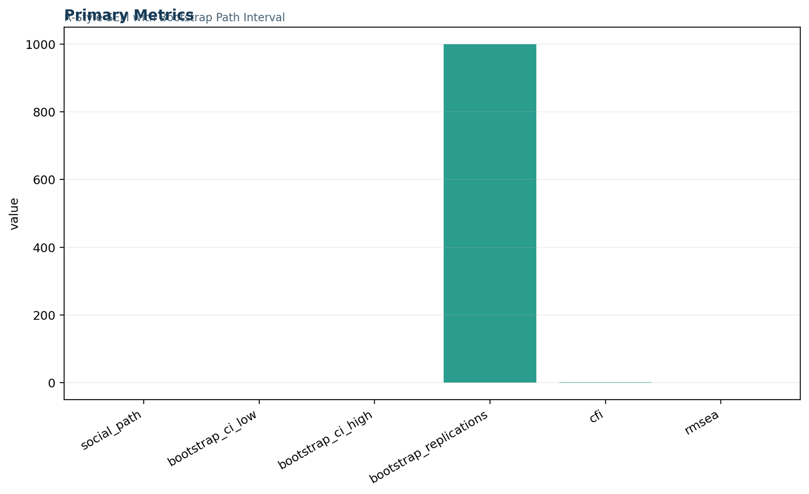
01 Sem-In-R Primary Metrics
This panel reconciles the headline estimate with its principal supporting values for SEM in R. Read CFI = 0.997823 beside TLI = 0.996735; the first quantity is not replaced by the second.
The chart is used to save the complete lavaan model string. Its interpretation remains valid only when the model syntax matches the theory. A visual pattern that conflicts with the saved table triggers re-estimation or relabeling of the specific chart, not a broad claim that the method has passed.
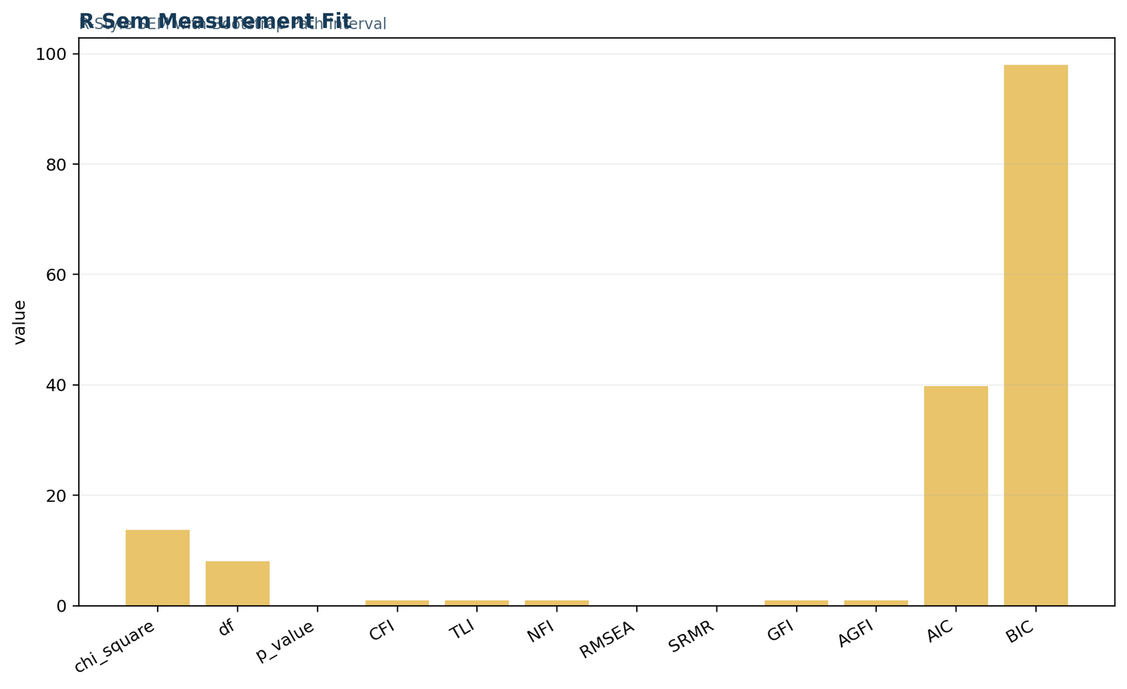
02 Sem-In-R R Sem Measurement Fit
This panel provides a visual diagnostic tied to the method’s exact decision rule for SEM in R. Read TLI = 0.996735 beside RMSEA = 0.020492; the first quantity is not replaced by the second.
The chart is used to call summary with fit.measures and standardized output. Its interpretation remains valid only when the data import preserves variable types. A visual pattern that conflicts with the saved table triggers re-estimation or relabeling of the specific chart, not a broad claim that the method has passed.
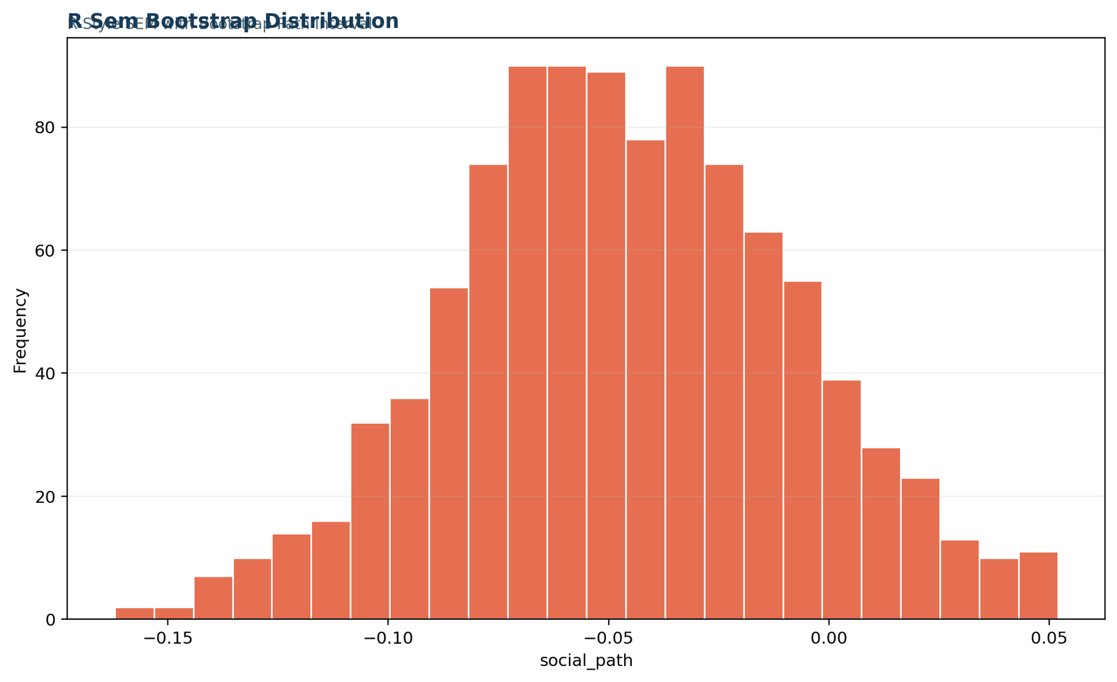
03 Sem-In-R R Sem Bootstrap Distribution
This panel shows sampling or resampling uncertainty around the reported estimate for SEM in R. Read RMSEA = 0.020492 beside SRMR = 0.035876; the first quantity is not replaced by the second.
The chart is used to extract exact values with fitMeasures and standardizedSolution. Its interpretation remains valid only when the estimator suits the scale and distribution. A visual pattern that conflicts with the saved table triggers re-estimation or relabeling of the specific chart, not a broad claim that the method has passed.
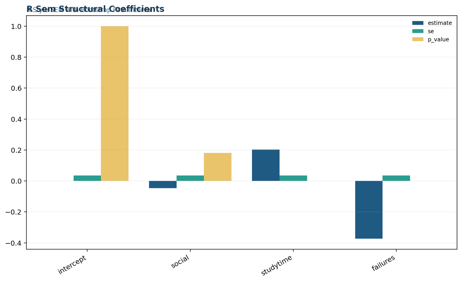
04 Sem-In-R R Sem Structural Coefficients
This panel shows the direction and relative magnitude of the declared structural relations for SEM in R. Read SRMR = 0.035876 beside Latent Education path = 0.382401; the first quantity is not replaced by the second.
The chart is used to inspect residuals and modification indices. Its interpretation remains valid only when the model is identified and converged. A visual pattern that conflicts with the saved table triggers re-estimation or relabeling of the specific chart, not a broad claim that the method has passed.
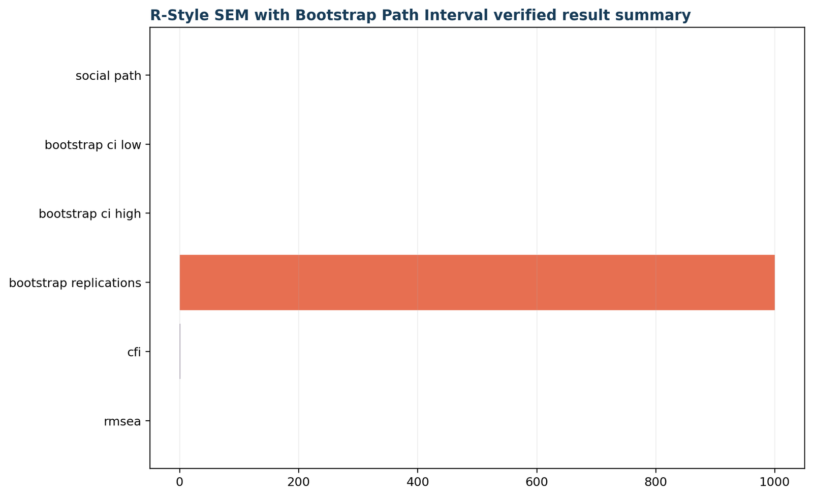
05 Sem-In-R Verified Result Summary
This panel reconciles the headline estimate with its principal supporting values for SEM in R. Read Latent Education path = 0.382401 beside Latent Social-Alcohol path = -0.477804; the first quantity is not replaced by the second.
The chart is used to record package and R versions. Its interpretation remains valid only when missingness is handled explicitly. A visual pattern that conflicts with the saved table triggers re-estimation or relabeling of the specific chart, not a broad claim that the method has passed.
01 Sem-In-R Primary Metrics
This panel reconciles the headline estimate with its principal supporting values for SEM in R. Read Latent Social-Alcohol path = -0.477804 beside Latent structural R squared = 0.167253; the first quantity is not replaced by the second.
The chart is used to avoid mixing semopy or AMOS numbers into the lavaan result. Its interpretation remains valid only when robust corrections are reported consistently. A visual pattern that conflicts with the saved table triggers re-estimation or relabeling of the specific chart, not a broad claim that the method has passed.
02 Sem-In-R R Sem Measurement Fit
This panel provides a visual diagnostic tied to the method’s exact decision rule for SEM in R. Read Latent structural R squared = 0.167253 beside PLS Education path = 0.282066; the first quantity is not replaced by the second.
The chart is used to save the complete lavaan model string. Its interpretation remains valid only when the model syntax matches the theory. A visual pattern that conflicts with the saved table triggers re-estimation or relabeling of the specific chart, not a broad claim that the method has passed.
03 Sem-In-R R Sem Bootstrap Distribution
This panel shows sampling or resampling uncertainty around the reported estimate for SEM in R. Read PLS Education path = 0.282066 beside PLS Social-Alcohol path = -0.197452; the first quantity is not replaced by the second.
The chart is used to call summary with fit.measures and standardized output. Its interpretation remains valid only when the data import preserves variable types. A visual pattern that conflicts with the saved table triggers re-estimation or relabeling of the specific chart, not a broad claim that the method has passed.
04 Sem-In-R R Sem Structural Coefficients
This panel shows the direction and relative magnitude of the declared structural relations for SEM in R. Read PLS Social-Alcohol path = -0.197452 beside PLS R squared = 0.120424; the first quantity is not replaced by the second.
The chart is used to extract exact values with fitMeasures and standardizedSolution. Its interpretation remains valid only when the estimator suits the scale and distribution. A visual pattern that conflicts with the saved table triggers re-estimation or relabeling of the specific chart, not a broad claim that the method has passed.
05 Sem-In-R Verified Result Summary
This panel reconciles the headline estimate with its principal supporting values for SEM in R. Read PLS R squared = 0.120424 beside PLS Q squared = 0.112273; the first quantity is not replaced by the second.
The chart is used to inspect residuals and modification indices. Its interpretation remains valid only when the model is identified and converged. A visual pattern that conflicts with the saved table triggers re-estimation or relabeling of the specific chart, not a broad claim that the method has passed.
SEM in R verification and sensitivity analysis
Six failure modes are checked against the formula, data, output, and charts.
The following diagnostics are not a general checklist. Each one targets a failure mode that can change the calculation or interpretation of SEM in R.
1. Save the complete lavaan model string
Begin by save the complete lavaan model string. For the lavaan SEM workflow, this operation directly connects CFI = 0.997823 with RMSEA = 0.020492. CFI = 0.997823 belongs to the declared covariance model and estimator; its baseline, complexity adjustment, or residual weighting must match the displayed formula.
The governing condition is that the model syntax matches the theory. If it fails, the primary coefficient may be attached to the wrong input object. The remedy is to correct the relevant coding, matrix, model, rotation, resampling, or panel denominator and rerun the calculation. This check also prevents confusion with SEM in AMOS, because AMOS represents the same model graphically, while lavaan provides text-based reproducibility and programmatic extraction.
2. Call summary with fit.measures and standardized output
Next, call summary with fit.measures and standardized output. For the lavaan SEM workflow, this operation directly connects TLI = 0.996735 with SRMR = 0.035876. TLI = 0.996735 belongs to the declared covariance model and estimator; its baseline, complexity adjustment, or residual weighting must match the displayed formula.
The governing condition is that the data import preserves variable types. If it fails, the companion statistic may no longer describe the same model or sample. The remedy is to correct the relevant coding, matrix, model, rotation, resampling, or panel denominator and rerun the calculation. This check also prevents confusion with Factor Analysis in R, because Factor-analysis workflows explore or estimate measurement structure; SEM in R adds structural regressions.
3. Extract exact values with fitMeasures and standardizedSolution
The third verification is to extract exact values with fitMeasures and standardizedSolution. For the lavaan SEM workflow, this operation directly connects RMSEA = 0.020492 with Latent Education path = 0.382401. RMSEA = 0.020492 expresses approximate discrepancy per degree of freedom and requires the corresponding confidence interval and estimator correction for complete reporting.
The governing condition is that the estimator suits the scale and distribution. If it fails, the decision boundary can move because the required quantity has changed. The remedy is to correct the relevant coding, matrix, model, rotation, resampling, or panel denominator and rerun the calculation. This check also prevents confusion with PLS-SEM, because lavaan primarily fits covariance-based SEM, not the iterative PLS composite algorithm.
4. Inspect residuals and modification indices
After the core arithmetic is stable, inspect residuals and modification indices. For the lavaan SEM workflow, this operation directly connects SRMR = 0.035876 with Latent Social-Alcohol path = -0.477804. SRMR = 0.035876 is the root mean square of standardized residuals; the average must be checked against the largest individual residual cells.
The governing condition is that the model is identified and converged. If it fails, software agreement can be artificial if unlike definitions are compared. The remedy is to correct the relevant coding, matrix, model, rotation, resampling, or panel denominator and rerun the calculation. This check also prevents confusion with SEM in AMOS, because AMOS represents the same model graphically, while lavaan provides text-based reproducibility and programmatic extraction.
5. Record package and R versions
A robustness review must record package and R versions. For the lavaan SEM workflow, this operation directly connects Latent Education path = 0.382401 with Latent structural R squared = 0.167253. Latent Education path = 0.382401 is a conditional model coefficient whose sign and magnitude are interpreted with uncertainty, collinearity, measurement quality, and design limits.
The governing condition is that missingness is handled explicitly. If it fails, a favorable average can conceal a local failure. The remedy is to correct the relevant coding, matrix, model, rotation, resampling, or panel denominator and rerun the calculation. This check also prevents confusion with Factor Analysis in R, because Factor-analysis workflows explore or estimate measurement structure; SEM in R adds structural regressions.
6. Avoid mixing semopy or AMOS numbers into the lavaan result
The final reconciliation should avoid mixing semopy or AMOS numbers into the lavaan result. For the lavaan SEM workflow, this operation directly connects Latent Social-Alcohol path = -0.477804 with PLS Education path = 0.282066. Latent Social-Alcohol path = -0.477804 is a conditional model coefficient whose sign and magnitude are interpreted with uncertainty, collinearity, measurement quality, and design limits.
The governing condition is that robust corrections are reported consistently. If it fails, the published conclusion can exceed the evidence actually reproduced. The remedy is to correct the relevant coding, matrix, model, rotation, resampling, or panel denominator and rerun the calculation. This check also prevents confusion with PLS-SEM, because lavaan primarily fits covariance-based SEM, not the iterative PLS composite algorithm.
| # | Verification operation | Condition protected | Saved quantity traced |
|---|---|---|---|
| 1 | save the complete lavaan model string | the model syntax matches the theory | CFI = 0.997823 |
| 2 | call summary with fit.measures and standardized output | the data import preserves variable types | TLI = 0.996735 |
| 3 | extract exact values with fitMeasures and standardizedSolution | the estimator suits the scale and distribution | RMSEA = 0.020492 |
| 4 | inspect residuals and modification indices | the model is identified and converged | SRMR = 0.035876 |
| 5 | record package and R versions | missingness is handled explicitly | Latent Education path = 0.382401 |
| 6 | avoid mixing semopy or AMOS numbers into the lavaan result | robust corrections are reported consistently | Latent Social-Alcohol path = -0.477804 |
SEM in R compared with related methods
Differences in estimand, formula, and conclusion determine the correct choice.
Method choice depends on the estimand, model, and data structure. These three comparisons explain why the post uses the SEM in R formula and output rather than a nearby procedure.
SEM in AMOS
AMOS represents the same model graphically, while lavaan provides text-based reproducibility and programmatic extraction.
In the current analysis, TLI = 0.996735 remains evidence for the lavaan SEM workflow; it is not relabeled as a SEM in AMOS result. TLI = 0.996735 belongs to the declared covariance model and estimator; its baseline, complexity adjustment, or residual weighting must match the displayed formula.
Factor Analysis in R
Factor-analysis workflows explore or estimate measurement structure; SEM in R adds structural regressions.
In the current analysis, RMSEA = 0.020492 remains evidence for the lavaan SEM workflow; it is not relabeled as a Factor Analysis in R result. RMSEA = 0.020492 expresses approximate discrepancy per degree of freedom and requires the corresponding confidence interval and estimator correction for complete reporting.
PLS-SEM
lavaan primarily fits covariance-based SEM, not the iterative PLS composite algorithm.
In the current analysis, SRMR = 0.035876 remains evidence for the lavaan SEM workflow; it is not relabeled as a PLS-SEM result. SRMR = 0.035876 is the root mean square of standardized residuals; the average must be checked against the largest individual residual cells.
How to report SEM in R
A complete result paragraph includes the value, analytical object, settings, and limitation.
Results paragraph
SEM in R was evaluated using the declared data, specification, and software settings. The primary result was CFI = 0.997823; TLI = 0.996735 and RMSEA = 0.020492 supplied supporting context. The lavaan model yields excellent fit and the stated latent paths. Full interpretation requires standardized loadings, residuals, factor correlations, R-squared, and estimator-specific fit measures from the same object.
The report then states the limitation explicitly: Different R packages and lavaan options can produce different corrections and fit indices. A script that merely prints a saved result is not a reproducible SEM, and exploratory modifications should not be presented as prespecified confirmation.
Settings that must accompany the result
the model syntax matches the theory; the data import preserves variable types; the estimator suits the scale and distribution; the model is identified and converged.
For SEM in R, these details identify the exact version of the analysis and make cross-software reconciliation possible.
Verification actions retained in the record
save the complete lavaan model string; call summary with fit.measures and standardized output; extract exact values with fitMeasures and standardizedSolution; inspect residuals and modification indices.
The final wording is revised only after those operations reproduce the saved values.
SEM in R decision scenarios
For SEM in R, worked conflicts show how the conclusion changes when an input, assumption, or supporting statistic fails.
Boundary-case interpretation: Save the complete lavaan model string
Consider a review in which CFI = 0.997823 is reproduced but TLI = 0.996735 is not. For the lavaan SEM workflow, the disagreement cannot be settled by averaging the two outputs because they describe different components of the analysis. The first action is to save the complete lavaan model string and verify that the model syntax matches the theory.
If the discrepancy persists, the analyst identifies whether the cause is coding, matrix construction, model identification, estimator, rotation, baseline definition, resampling, or panel denominator. The result is compared with SEM in AMOS only for method selection: AMOS represents the same model graphically, while lavaan provides text-based reproducibility and programmatic extraction. The published conclusion remains The lavaan model yields excellent fit and the stated latent paths. Full interpretation requires standardized loadings, residuals, factor correlations, R-squared, and estimator-specific fit measures from the same object.
Input-definition sensitivity: Call summary with fit.measures and standardized output
Consider a review in which RMSEA = 0.020492 is reproduced but SRMR = 0.035876 is not. For the lavaan SEM workflow, the disagreement cannot be settled by averaging the two outputs because they describe different components of the analysis. The first action is to call summary with fit.measures and standardized output and verify that the data import preserves variable types.
If the discrepancy persists, the analyst identifies whether the cause is coding, matrix construction, model identification, estimator, rotation, baseline definition, resampling, or panel denominator. The result is compared with Factor Analysis in R only for method selection: Factor-analysis workflows explore or estimate measurement structure; SEM in R adds structural regressions. The published conclusion remains The lavaan model yields excellent fit and the stated latent paths. Full interpretation requires standardized loadings, residuals, factor correlations, R-squared, and estimator-specific fit measures from the same object.
Software-definition reconciliation: Extract exact values with fitMeasures and standardizedSolution
Consider a review in which Latent Education path = 0.382401 is reproduced but Latent Social-Alcohol path = -0.477804 is not. For the lavaan SEM workflow, the disagreement cannot be settled by averaging the two outputs because they describe different components of the analysis. The first action is to extract exact values with fitMeasures and standardizedSolution and verify that the estimator suits the scale and distribution.
If the discrepancy persists, the analyst identifies whether the cause is coding, matrix construction, model identification, estimator, rotation, baseline definition, resampling, or panel denominator. The result is compared with PLS-SEM only for method selection: lavaan primarily fits covariance-based SEM, not the iterative PLS composite algorithm. The published conclusion remains The lavaan model yields excellent fit and the stated latent paths. Full interpretation requires standardized loadings, residuals, factor correlations, R-squared, and estimator-specific fit measures from the same object.
Local-chart conflict: Inspect residuals and modification indices
Consider a review in which Latent structural R squared = 0.167253 is reproduced but PLS Education path = 0.282066 is not. For the lavaan SEM workflow, the disagreement cannot be settled by averaging the two outputs because they describe different components of the analysis. The first action is to inspect residuals and modification indices and verify that the model is identified and converged.
If the discrepancy persists, the analyst identifies whether the cause is coding, matrix construction, model identification, estimator, rotation, baseline definition, resampling, or panel denominator. The result is compared with SEM in AMOS only for method selection: AMOS represents the same model graphically, while lavaan provides text-based reproducibility and programmatic extraction. The published conclusion remains The lavaan model yields excellent fit and the stated latent paths. Full interpretation requires standardized loadings, residuals, factor correlations, R-squared, and estimator-specific fit measures from the same object.
Alternative-method challenge: Record package and R versions
Consider a review in which PLS Social-Alcohol path = -0.197452 is reproduced but PLS R squared = 0.120424 is not. For the lavaan SEM workflow, the disagreement cannot be settled by averaging the two outputs because they describe different components of the analysis. The first action is to record package and R versions and verify that missingness is handled explicitly.
If the discrepancy persists, the analyst identifies whether the cause is coding, matrix construction, model identification, estimator, rotation, baseline definition, resampling, or panel denominator. The result is compared with Factor Analysis in R only for method selection: Factor-analysis workflows explore or estimate measurement structure; SEM in R adds structural regressions. The published conclusion remains The lavaan model yields excellent fit and the stated latent paths. Full interpretation requires standardized loadings, residuals, factor correlations, R-squared, and estimator-specific fit measures from the same object.
Replication and reporting decision: Avoid mixing semopy or AMOS numbers into the lavaan result
Consider a review in which PLS Q squared = 0.112273 is reproduced but Observed path R squared = 0.850714 is not. For the lavaan SEM workflow, the disagreement cannot be settled by averaging the two outputs because they describe different components of the analysis. The first action is to avoid mixing semopy or AMOS numbers into the lavaan result and verify that robust corrections are reported consistently.
If the discrepancy persists, the analyst identifies whether the cause is coding, matrix construction, model identification, estimator, rotation, baseline definition, resampling, or panel denominator. The result is compared with PLS-SEM only for method selection: lavaan primarily fits covariance-based SEM, not the iterative PLS composite algorithm. The published conclusion remains The lavaan model yields excellent fit and the stated latent paths. Full interpretation requires standardized loadings, residuals, factor correlations, R-squared, and estimator-specific fit measures from the same object.
Boundary-case interpretation: Save the complete lavaan model string
Consider a review in which Observed path adjusted R squared = 0.849084 is reproduced but Observed path RMSE = 1.247283 is not. For the lavaan SEM workflow, the disagreement cannot be settled by averaging the two outputs because they describe different components of the analysis. The first action is to save the complete lavaan model string and verify that the model syntax matches the theory.
If the discrepancy persists, the analyst identifies whether the cause is coding, matrix construction, model identification, estimator, rotation, baseline definition, resampling, or panel denominator. The result is compared with SEM in AMOS only for method selection: AMOS represents the same model graphically, while lavaan provides text-based reproducibility and programmatic extraction. The published conclusion remains The lavaan model yields excellent fit and the stated latent paths. Full interpretation requires standardized loadings, residuals, factor correlations, R-squared, and estimator-specific fit measures from the same object.
Input-definition sensitivity: Call summary with fit.measures and standardized output
Consider a review in which G2 observed coefficient = 0.887127 is reproduced but CFI = 0.997823 is not. For the lavaan SEM workflow, the disagreement cannot be settled by averaging the two outputs because they describe different components of the analysis. The first action is to call summary with fit.measures and standardized output and verify that the data import preserves variable types.
If the discrepancy persists, the analyst identifies whether the cause is coding, matrix construction, model identification, estimator, rotation, baseline definition, resampling, or panel denominator. The result is compared with Factor Analysis in R only for method selection: Factor-analysis workflows explore or estimate measurement structure; SEM in R adds structural regressions. The published conclusion remains The lavaan model yields excellent fit and the stated latent paths. Full interpretation requires standardized loadings, residuals, factor correlations, R-squared, and estimator-specific fit measures from the same object.
Software-definition reconciliation: Extract exact values with fitMeasures and standardizedSolution
Consider a review in which TLI = 0.996735 is reproduced but RMSEA = 0.020492 is not. For the lavaan SEM workflow, the disagreement cannot be settled by averaging the two outputs because they describe different components of the analysis. The first action is to extract exact values with fitMeasures and standardizedSolution and verify that the estimator suits the scale and distribution.
If the discrepancy persists, the analyst identifies whether the cause is coding, matrix construction, model identification, estimator, rotation, baseline definition, resampling, or panel denominator. The result is compared with PLS-SEM only for method selection: lavaan primarily fits covariance-based SEM, not the iterative PLS composite algorithm. The published conclusion remains The lavaan model yields excellent fit and the stated latent paths. Full interpretation requires standardized loadings, residuals, factor correlations, R-squared, and estimator-specific fit measures from the same object.
Local-chart conflict: Inspect residuals and modification indices
Consider a review in which SRMR = 0.035876 is reproduced but Latent Education path = 0.382401 is not. For the lavaan SEM workflow, the disagreement cannot be settled by averaging the two outputs because they describe different components of the analysis. The first action is to inspect residuals and modification indices and verify that the model is identified and converged.
If the discrepancy persists, the analyst identifies whether the cause is coding, matrix construction, model identification, estimator, rotation, baseline definition, resampling, or panel denominator. The result is compared with SEM in AMOS only for method selection: AMOS represents the same model graphically, while lavaan provides text-based reproducibility and programmatic extraction. The published conclusion remains The lavaan model yields excellent fit and the stated latent paths. Full interpretation requires standardized loadings, residuals, factor correlations, R-squared, and estimator-specific fit measures from the same object.
Alternative-method challenge: Record package and R versions
Consider a review in which Latent Social-Alcohol path = -0.477804 is reproduced but Latent structural R squared = 0.167253 is not. For the lavaan SEM workflow, the disagreement cannot be settled by averaging the two outputs because they describe different components of the analysis. The first action is to record package and R versions and verify that missingness is handled explicitly.
If the discrepancy persists, the analyst identifies whether the cause is coding, matrix construction, model identification, estimator, rotation, baseline definition, resampling, or panel denominator. The result is compared with Factor Analysis in R only for method selection: Factor-analysis workflows explore or estimate measurement structure; SEM in R adds structural regressions. The published conclusion remains The lavaan model yields excellent fit and the stated latent paths. Full interpretation requires standardized loadings, residuals, factor correlations, R-squared, and estimator-specific fit measures from the same object.
Replication and reporting decision: Avoid mixing semopy or AMOS numbers into the lavaan result
Consider a review in which PLS Education path = 0.282066 is reproduced but PLS Social-Alcohol path = -0.197452 is not. For the lavaan SEM workflow, the disagreement cannot be settled by averaging the two outputs because they describe different components of the analysis. The first action is to avoid mixing semopy or AMOS numbers into the lavaan result and verify that robust corrections are reported consistently.
If the discrepancy persists, the analyst identifies whether the cause is coding, matrix construction, model identification, estimator, rotation, baseline definition, resampling, or panel denominator. The result is compared with PLS-SEM only for method selection: lavaan primarily fits covariance-based SEM, not the iterative PLS composite algorithm. The published conclusion remains The lavaan model yields excellent fit and the stated latent paths. Full interpretation requires standardized loadings, residuals, factor correlations, R-squared, and estimator-specific fit measures from the same object.
SEM in R downloads and reproducibility files
All linked files belong to the same analysis and remain on onlineinternetcafe.com.
The four files belong to one SEM in R analysis. Their primary values, variable order, method settings, and chart labels must agree; a mismatch is resolved in the source calculation before the WordPress draft is published.
SEM in R frequently asked questions
Answers use the worked result and the exact method boundary.
What does SEM in R measure?
SEM in R is implemented here with lavaan syntax that declares latent variables using =~, regressions using ~, and covariances using ~~ where justified. The script, estimator, missing-data rule, and requested standardized output make the analysis reproducible.
What is the main result in this SEM in R analysis?
CFI = 0.997823. The lavaan model yields excellent fit and the stated latent paths. Full interpretation requires standardized loadings, residuals, factor correlations, R-squared, and estimator-specific fit measures from the same object.
What does the result not prove?
Different R packages and lavaan options can produce different corrections and fit indices. A script that merely prints a saved result is not a reproducible SEM, and exploratory modifications should not be presented as prespecified confirmation.
Which supporting value should be reported with the primary result?
For SEM in R, tLI = 0.996735 is the first companion quantity. TLI = 0.996735 belongs to the declared covariance model and estimator; its baseline, complexity adjustment, or residual weighting must match the displayed formula.
Which assumption is most likely to change the interpretation?
The first requirement is that the model syntax matches the theory. The result is recomputed if that condition is not satisfied.
What is the most important numerical verification?
The analyst must save the complete lavaan model string. That operation traces CFI = 0.997823 to the formula and saved inputs.
Why can software packages disagree on SEM in R?
Disagreement can arise because the data import preserves variable types or because the packages implement different estimators, matrices, baselines, rotations, standardizations, bootstrap rules, or coefficient definitions. Matching labels alone is not enough.
How is SEM in R different from SEM in AMOS?
AMOS represents the same model graphically, while lavaan provides text-based reproducibility and programmatic extraction.
How should a chart be interpreted?
For SEM in R, each chart is tied to a named output such as RMSEA = 0.020492. It supports a local calculation or diagnostic and does not replace the full numerical result.
How should SEM in R be reported?
Report CFI = 0.997823, the required supporting quantities, sample or panel size, exact method settings, and this qualified conclusion: The lavaan model yields excellent fit and the stated latent paths. Full interpretation requires standardized loadings, residuals, factor correlations, R-squared, and estimator-specific fit measures from the same object.